Lecture 01:

Welcome to the course. This is an introduction to neural networks and deep learning, covering the fundamentals you need to understand modern AI systems.

I've been teaching this deep learning course for about five years now. Let's start with the big picture: what can neural networks actually do? The range of applications has exploded in recent years, and the answer might surprise you.

I think this is a really interesting course because it covers the foundation for modern AI. You're going to see topics on large language models and generative AI, but this is really about the fundamentals underneath all of that. Not everything we do is generative AI, so a lot of what you'll learn here will be practically useful in your careers. Today, I'm going to do a general introduction to neural networks to motivate some concepts -- things you may have seen before, but I'm going to add context to get you thinking differently. Modern deep learning thinks very differently from how you may have learned to model using traditional statistics.

My day job is as a senior director at a major bank, where I lead a team of around 100 people building high-value AI use cases across the enterprise. A lot of what I cover in these lectures draws directly from that hands-on experience shipping production AI systems. My goal with this course goes beyond just teaching the theory -- it's grounded in practical experience building real systems.

Beyond the lectures themselves, what I hope to give you is more context on how to think about these things practically in industry. The gap between academic deep learning and production deep learning is real, and I want to bridge that gap wherever I can.

I used to have a slide on image generation, but that's so five years ago. Now we have these amazing video generation models. You type in a detailed prompt, and it generates a full video from that description. We're still in the infancy of these tools, and they're going to get a lot better. What's remarkable is how quickly we went from barely generating coherent images to producing photorealistic video -- it speaks to the pace of progress in this field.

My wife is a physician, so this is a running joke at home -- "soon we won't need you, AI will solve all these problems." It's a nuanced topic, but depending on where you look, AI is already outperforming doctors on certain diagnostic measures. The nature of even highly specialized jobs is going to change. We've got to be prepared for that one way or another.

Everyone knows ChatGPT, and hopefully some of you are at least a little concerned: am I going to have a job in five or ten years? It's a real question. I've revised a lot of material in the last couple of years because of the generative AI boom. The latest models -- O1, O3 from OpenAI -- are off the charts, performing better than the average PhD on PhD-level exams. On software engineering, a couple of years ago these models could barely write a simple function. Now they can write entire programs with minimal guidance. It's changing the nature of our jobs, even for people building AI systems like myself. The pace of improvement is stunning, and we don't know exactly where it leads.

Neural networks and traditional machine learning have been used in a lot of less glamorous use cases for a long time. Across many industries -- finance, healthcare, retail, manufacturing -- there are countless problems that benefit from these tools. Not everyone's going to work on self-driving cars, but I'd bet most of you will work on something in these ranges. Having the tools of modern AI and deep learning will be useful when you tackle these problems.

That's the motivation for why we want to learn this. Now I want to give you a different point of view -- I come from a machine learning background, and we have a very different view on modeling compared to, say, an economics or statistics perspective. A lot of industry is shifting towards this view, and for larger-scale problems, it's a lot more practical. Here's a simple way to think about how computing has shifted with machine learning. Traditional computing: you write a program, feed it inputs, and it produces outputs. That's coding -- a very simple model. Machine learning is a different paradigm. You're no longer telling the computer how to solve the problem. You're giving it data -- input examples and expected outputs -- and letting it figure out the solution.

With machine learning, I'm giving the computer a dataset -- input examples and expected outputs. I'm not telling the machine how to do it. Through a machine learning algorithm, it generates not outputs directly, but a program -- which we call a model. This model can then take new inputs and predict new outputs. It's a fundamentally different way of building software.

What's remarkable is that many problems AI solves today are ones we genuinely don't know how to write programs for. The only way we can solve them is by plugging data into a machine learning algorithm and letting it learn. Take email spam detection as a concrete example. Writing an explicit spam filter is incredibly hard -- you might start with a blacklist of words, but spammers adapt constantly. You could never keep up manually. Yet since the late '90s, machine learning has handled this beautifully. You provide labeled examples of spam and not-spam, and the algorithm adjusts its own parameters to classify correctly. This is the core promise: give it data, and it solves the problem itself.

Andrej Karpathy, former director of AI at Tesla and early OpenAI researcher, articulated this through his "Software 2.0" thesis about a decade ago. He visualized the space of all solvable problems as concentric circles. Software 1.0 -- traditional code -- can only solve problems where we can explicitly specify the solution. Software 2.0, powered by machine learning and deep learning, opens up a vastly larger space. We don't need to tell the computer how to solve the problem -- we just need to specify what the inputs and outputs should look like and curate the right data. Of course, Software 1.0 isn't going away. As for Software 3.0, many point to AI agents, but that vision is still maturing.

Let me clarify the terminology hierarchy. AI is the broadest category -- any machine that mimics human intelligence. Early AI in the 1950s was symbolic: logic, search, rule-based systems. As computing power and data grew, statistical learning took over. Machine learning is the subset of AI that learns from data. Deep learning, using neural networks, is a subset of machine learning. And generative AI -- large language models, foundation models -- sits inside deep learning. Use these terms correctly, even though most people don't.

You should be using generative AI. Everyone's going to use it, so I want you to get experience with it. The important thing is that you write your own prompts and develop your own intuition for how these tools work. In ten years, everyone will be using this the same way everyone uses Google or Wikipedia today. You're also responsible for the validity of what the AI produces -- don't just copy the output. Read it over, apply judgment, make sure it's correct in context. That's your responsibility as a practitioner.

Historically, the biggest enabler of modern AI is computing power. Moore's Law -- transistor counts doubling roughly every 18 to 24 months -- creates an exponential curve. People expected it to die in the '90s, the 2000s, the 2010s, yet it persists. Almost every AI advance rides this wave of increasing compute. Without the raw computational power, none of the algorithms we had sitting on the shelf for decades would have become practical.

The second enabler is data -- massive amounts of it, especially from the internet. Machine learning is hungry for examples, and the explosion of digital data over the last two decades has fed that hunger. More data means better models, and the internet has provided an unprecedented scale of training data for everything from language to images to video.

One of the really scary things recently is deep fakes. These are getting better and better. I actually downloaded an app called Captions and made a video of my brother saying how great I was -- it was hilarious. He was like, "what the hell?" And now it's literally five bucks for a month of the app. Anyone can do it. The implications are genuinely concerning when you think about trust and verification in a world where anyone can generate convincing fake video.

Self-driving cars have actually surprised me. For a long time, I was pessimistic about them, but you can go to San Francisco or LA right now and call a Waymo -- totally self-driving across the entire city. A lot of that capability is driven by neural networks and modern AI. This is distinct from Tesla's autopilot, which uses AI but isn't at the same level of autonomous driving as Waymo. We're also using AI to predict how proteins interact, which is speeding up research in biology and medicine. The hope is to find better drugs for cancer and other diseases. It's not just affecting digital things anymore -- it's starting to impact the biological world too.

Why are neural networks so effective? Consider what we used to do. Back in the 2000s, image recognition required manual feature extraction. We used image filters called kernels -- small grids of numbers applied through discrete convolution across an image's pixels. These kernels could blur, sharpen, or detect edges, similar to Photoshop filters. The workflow was painfully manual: pick kernels, extract features, then feed those features into a simpler model like an SVM. You were essentially guessing which features might be useful. The breakthrough came in 2012 with AlexNet -- instead of hand-picking a few kernels, let the neural network learn what kernels it needs. Use tens of thousands of them and let the network figure out the right values.

This automatic feature learning creates a natural hierarchy that nobody programmed in. The lower layers of a neural network learn to detect fundamental visual elements -- horizontal edges, vertical edges, diagonal edges, slight curves. These are the basic building blocks of images. The middle layers combine those simple features into recognizable components: eyes, noses, mouths, wheels. The top layers assemble those components into full object recognition. This hierarchy emerged purely from learning on data with sufficient compute. No one told the network to look for edges first, then parts, then whole objects. This is one of the greatest strengths of neural networks: they automatically learn the right feature representations at multiple levels of abstraction.

The third enabler is research -- better algorithms. Though many core techniques like RNNs and CNNs existed since the late '90s, we just lacked the compute to make them useful. It's the combination of all three -- compute, data, and research -- that created the explosion we're seeing now. No single factor alone would have been sufficient.

Neural networks are particularly powerful because they scale. Just add layers or neurons, and the network gains more flexibility to model complex data distributions. The underlying algorithm is simple, and given enough compute, memory, and data, you can make them arbitrarily large. That scalability is exactly what the field has exploited -- it's also why NVIDIA's stock has skyrocketed, because everyone needs GPUs for this compute.

Parameters are the learnable coefficients in a model -- analogous to the slope and intercept in linear regression. One key measure of model complexity is parameter count, since each one must be learned during training. The progression has been staggering: classical statistical models typically use fewer than 100 parameters, LeNet in 1998 used about 60,000, and the growth has followed an aggressive exponential curve up through GPT-3 and GPT-4, which exceeds a trillion parameters. Interestingly, researchers who saw GPT-2 recognized its potential, and GPT-3 confirmed the scaling trend, but it took ChatGPT's interface to reveal just how powerful these large models could be.

The field has recently shifted paradigms around compute allocation. Up until GPT-4, the dominant approach was simply scaling up parameters and training data. But anecdotally, the major labs started seeing diminishing returns in 2024, possibly because we've exhausted high-quality training data. The new paradigm is test-time compute: instead of spending all your compute on training, you let the model spend more computation during inference -- essentially giving it time to "think." This is the principle behind models like O1, O3, and DeepSeek's R1. We appear to be in a fundamentally different regime now where the quality of reasoning at inference time matters as much as raw model size.

At the beginning of each section, I present a set of review questions that capture the main ideas I want you to learn. I show the questions upfront before the lecture content so you know what to focus on while listening. Then at the end of each section, we review them verbally. This repeated exposure -- preview, lecture, review -- is designed to maximize retention of the core concepts. The marks are just a byproduct of genuine learning.

In machine learning, I think of models as function approximators. The goal is to learn a function that maps inputs to outputs based on training data. A good function approximator needs to be flexible enough to capture complex patterns while remaining trainable through optimization. Neural networks excel here because they can approximate virtually any continuous function given sufficient width and depth -- this is related to the universal approximation theorem. We need something that can represent nonlinear relationships, that's differentiable so we can use gradient-based optimization, and that scales well with more parameters and data. Neural networks satisfy all of these criteria.

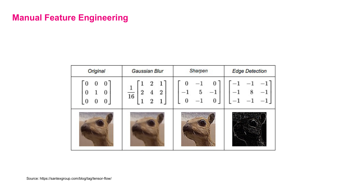
To understand why neural networks work so well, start with the simplest function approximator: a linear function. Linear models map inputs to outputs through weighted sums -- straightforward and easy to optimize. But they can only capture linear relationships. Virtually no interesting real-world problem is truly linear. Images, language, speech -- these all involve deeply nonlinear patterns. The 1969 XOR problem demonstrated that a single-layer perceptron -- essentially a linear classifier -- couldn't solve even this trivially nonlinear problem. The solution involves adding more layers and nonlinear activation functions.

This slide introduces the idea of looking at local neighborhoods of pixels to compute useful features. The technique examines a 3x3 area around each center pixel and computes a weighted average over that neighborhood. This operation is called a discrete finite-length convolution, and it's fundamental to how modern image recognition works. Rather than treating each pixel independently, convolutions capture local spatial structure -- edges, textures, patterns. We'll dig into convolutions in much more detail later, since they form the backbone of convolutional neural networks. For now, the key takeaway is that moving beyond per-pixel operations to local neighborhood operations gives us a more powerful class of functions for processing images.

Inputs have many names -- features, regressors, covariates, independent variables -- and you should use these interchangeably depending on your audience. Outputs are called observations, response variables, labels, or target variables. The simplest function approximator is a line with two parameters -- intercept and slope -- and training means finding the best values for those. But linear models are rigid and can't capture complex patterns. We can add polynomial features like x² and x³ for more flexibility, but that requires manual feature engineering across potentially hundreds of variables. A neural network solves this elegantly: a five-layer, 500-unit network with a million parameters can fit complex patterns without hand-crafting any features.

The hidden layer function involves a matrix multiplication -- a weight matrix times the input vector -- plus a bias vector, followed by an element-wise activation function. The weight matrix contains d times n parameters, and the bias vector adds more on top of that. Even for a single hidden layer, we're already introducing a substantial number of learnable parameters compared to simple linear models.

The weight matrix is a full matrix of d times n parameters, and the bias is a vector of additional parameters. You can already see we're adding a lot of parameters compared to the simple linear model. This is exactly the mechanism that gives neural networks their flexibility -- each layer introduces its own weights and biases that training needs to optimize. The sheer number of learnable parameters is what enables the network to capture complex patterns in the data.

By composing multiple hidden layers together -- five layers of 500 units each -- we get a neural network with a million parameters, all from a single input feature x. The resulting approximation fits the data far better than any polynomial, though it likely overfits in this case. The key takeaway: neural networks are excellent function approximators because they're easy to scale. A parameter is any number in the model we need to learn during training. Linear functions are poor approximators because they have too few parameters and degrees of freedom. Neural networks overcome this through their layered structure combined with scalability.

Section 2 covers the basics of feed-forward neural networks. I use the same structure: questions at the start, lecture content, then review at the end. Knowing the questions in advance helps you actively listen for key concepts rather than passively absorbing information. The three key questions for this section are: What is a parameter? Why are linear functions poor function approximators? And why are neural networks good function approximators?

Function approximation is the most practical lens for understanding machine learning. Going back to high school math, a function maps inputs from a domain to outputs in a range, where each input produces exactly one output. In supervised machine learning, we have data points with inputs and corresponding outputs, and our goal is to learn a function that approximates the true relationship between them. This perspective cuts through the many different ways people talk about machine learning and gives us a concrete, actionable framework. The quality of our approximation depends entirely on the class of functions we choose -- which is exactly why we need to understand the limitations of linear functions and the power of neural networks.

A perceptron is simply a linear function with a non-linear activation function applied on top. Without that non-linearity, stacking linear layers would still only represent a linear function -- the activation function is what makes neural networks special. Historically, sigmoid and tanh were the main activation functions, partly because their derivatives are simple to compute. But we've since found faster architectures, and ReLU has become the standard. ReLU is simple: if the input is negative, return zero; if positive, pass the value through unchanged. It's non-linear and its derivative is trivially easy to compute. My general advice: start with ReLU -- it works well in most cases -- and only change it if you need to.

One of the big ideas in deep learning is that stacking more non-linear perceptrons lets you model increasingly complicated functions. This is the core insight behind scaling neural networks. To build intuition, consider a simple network diagram. The first layer -- the input nodes -- just represents your features. These aren't computation units; they simply pass your input data into the network. Understanding this distinction is important: inputs are not neurons performing calculations, they're just the entry point for your data.

In a neural network diagram, the input nodes on the left represent your features -- they don't perform any computation. Everything between the input and output layers is called a hidden layer. Each node in the hidden and output layers is a neuron or perceptron, performing a linear combination plus non-linear activation. So when reading network diagrams: input nodes are data entry points, hidden layer neurons do the actual computation and pattern recognition, and output neurons produce the final predictions.

Now let's add more perceptrons. Here's a network with two inputs, one hidden layer of three neurons, and two outputs. The depth is two -- input layer doesn't count. Width is [2, 3, 2]. To count parameters: the first weight matrix is 3x2 = 6 weights, plus 3 biases. The second matrix is 2x3 = 6 weights, plus 2 biases. Total: (32+3) + (23+2) = 17 parameters. The compact form is just W2 times sigma of (W1*x + b1) plus b2. Each layer introduces its own weight matrix and bias vector, and the activation function sigma goes between them. This notation scales to any number of layers.

Now let's add more layers. Here we have 3 inputs, 3 hidden layers of 4 neurons each, and 3 outputs. Depth is 4, width is [3, 4, 4, 4, 3], and the parameter count is (43+4) + (44+4) + (44+4) + (34+3) = 71. Notice the function is just nested compositions: W4 times sigma of W3 times sigma of W2 times sigma of (W1*x + b1) + b2) + b3) + b4. Each layer adds its own weight matrix and bias, with an activation function in between. The pattern is always the same -- you're just stacking more of them.

And this is what a "deep" neural network looks like. Five inputs, 10 hidden layers of 10 neurons each, 5 outputs. Depth is 11, and the parameter count is 1,105. The word "deep" in deep learning literally means many layers -- and the definition of what counts as "deep" keeps shifting as we build bigger networks. What used to be considered deep is now shallow by modern standards. The key insight is that each additional layer gives the network another opportunity to learn more abstract representations. And because the underlying computation is just matrix multiplications and activation functions, it scales straightforwardly with more compute.

How do we define the output perceptrons? The output neurons model the y values -- your labels or targets. The activation function on the output layer should match your response variable. Key considerations: is it a regression or classification problem? What's the range of the output variable? Is it discrete or continuous? We'll look at four common activation functions for output units: identity (for unbounded real-valued outputs), ReLU (for positive real-valued outputs), sigmoid (for binary classification), and softmax (for multi-class classification). The choice of output activation determines what kind of predictions your network can make.

For linear output, we use the identity activation -- the output is just the raw value from the linear combination. This is what you'd use for regression problems where the target can be any real number. For positive real-valued output, we use ReLU on the output unit, which clips negative values to zero. This makes sense when your target is something like a price or a count -- values that can't be negative. The simple network on this slide has two inputs, one hidden neuron, and one output. Depth is two, width is [2, 1, 1]. Count the parameters: two weights into the hidden unit plus one bias, then one weight to the output plus one bias -- that's five parameters total.

For binary output, you'd use a sigmoid activation on the output unit, which squashes the result to a probability between zero and one. This is what you want for yes/no classification problems. For categorical output with multiple classes, you'd use softmax across multiple output units, ensuring the outputs sum to one and can be interpreted as class probabilities. The choice of output activation directly determines what kind of prediction your network can make -- it's one of the key architectural decisions you need to get right.

As we review Section 2, I want to highlight something about notation. I deliberately wrote out every individual weight -- W111, W112, and so on -- so it's obvious what's happening. But going forward, and in most neural network literature, people use matrix form directly, compressing all those individual weights into a single matrix W1. You need to get comfortable with this notation because as networks get larger, you simply cannot write out every weight explicitly. Being able to look at a matrix expression and mentally unpack it into the individual operations at each neuron and layer is a key skill for reading papers and understanding deep learning frameworks.

To summarize Section 2: how do you calculate the number of parameters in a neural network? It's the number of connections between layers plus the number of bias parameters -- one bias per neuron in the hidden and output layers. A common mistake is thinking the parameter count equals the number of neurons. You need to count every edge between adjacent layers, then add the biases. For a layer with m inputs connecting to n neurons, you get m times n weights plus n biases. This formula scales to any architecture. Understanding parameter counting is fundamental because it tells you the model's capacity and helps you reason about overfitting, computational requirements, and memory usage.