Lecture 08: Attention and Transformers

Today we're continuing with more advanced topics: attention, self-attention, and Transformers. The Transformer architecture is the backbone of large language models today, so we need to understand how it works. Obviously we could spend an entire course on this, but I want to get across the main ideas so that when you're working in this space, you'll have a solid intuition for the constraints and mechanics involved. A quick note on final projects: proposals are due this Friday. The key idea is to learn something new and teach it back to the class. Don't pick the most complicated topic possible — pick something you can finish in three or four weeks. Make sure you have a well-formulated problem with a non-trivial dataset, and go beyond what we covered in class. Getting state-of-the-art results isn't the point. Even negative results teach you something valuable. The experiment section is about playing with the model, changing hyperparameters, comparing approaches, and sharing what you learned.

The fundamental limitation of the encoder-decoder architecture is that information bottleneck — trying to compress everything into a single context vector and then decode from it. Even if we could pack all the information in, decoding that one vector is itself a huge problem. So how do we fix this? We introduce an attention mechanism between the encoder and decoder. Instead of passing just the final hidden state to the decoder, we pass the hidden state from every intermediate step. If we have ten tokens, we pass ten vectors. This removes the information bottleneck. Then, instead of using those vectors as a single initial state for the decoder, we create unique context vectors that get fed into each decoding step individually. The attention mechanism decides, for each decoding step, which encoder hidden states to emphasize. So when decoding the first output token, attention looks at all the encoder states and determines which ones are most relevant for that specific step. Each subsequent decoding step gets its own tailored context, relieving the decoder of the burden of extracting everything from one compressed representation.

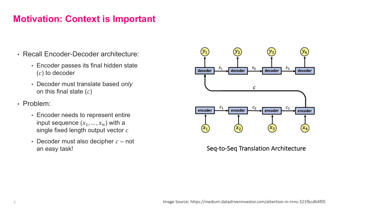
Recall the basic encoder-decoder architecture for sequence-to-sequence tasks like machine translation. The encoder processes the entire input sequence and passes its final hidden state c to the decoder, which must then generate the output based solely on that single fixed-length vector. The problem is twofold: first, the encoder must compress the entire input sequence into one vector, which becomes increasingly difficult as sequences get longer. Second, the decoder must extract all relevant information from that single compressed representation — not an easy task. This information bottleneck is the core limitation. For short sequences it works reasonably well, but for longer inputs the quality degrades because too much information is lost in compression. The attention mechanism was designed specifically to address this bottleneck.

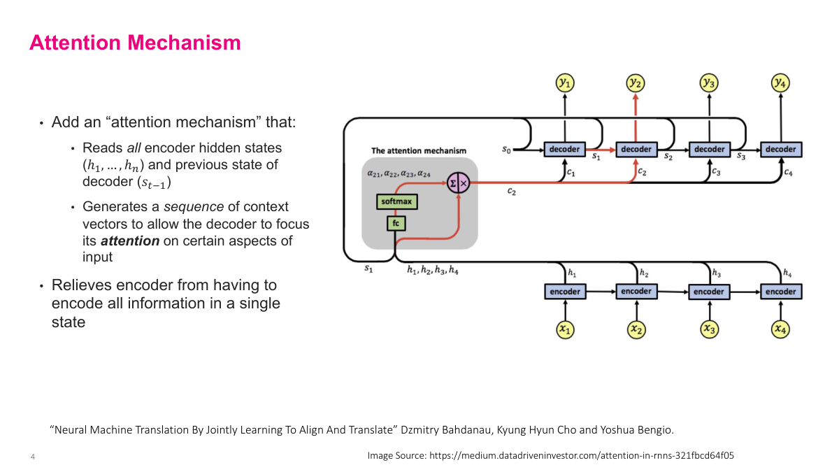
The attention mechanism solves the information bottleneck by reading all encoder hidden states, not just the final one. It takes every hidden state h1 through hn from the encoder along with the previous decoder state s_{t-1}, and generates a sequence of context vectors — one for each decoding step. This allows the decoder to focus its attention on different parts of the input at each step. The mechanism uses a fully connected layer followed by softmax to produce attention weights, which determine how much each encoder hidden state contributes to the current context vector. For the first decoding step, it combines s0 with all encoder states to produce c1. Then s1 wraps around with the encoder states to produce c2, and so on. This relieves the encoder from having to compress everything into a single state, since the decoder can now selectively attend to the most relevant parts of the input at each step. This architecture comes from the landmark Bahdanau et al. paper on neural machine translation.

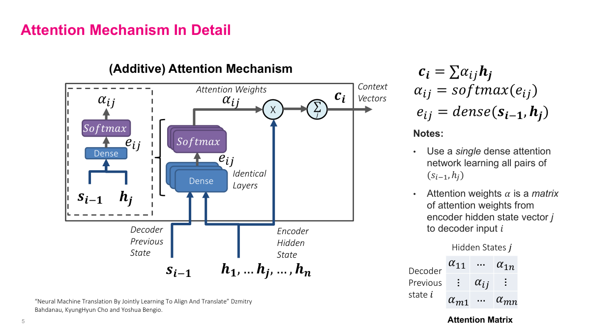
This slide breaks down the additive attention mechanism in detail. The core computation has three steps. First, energy scores e_ij are computed by passing the previous decoder state s_{i-1} and each encoder hidden state h_j through a dense layer. Second, these energy scores go through a softmax to produce the attention weights alpha_ij, which sum to one across all encoder positions. Third, the context vector c_i is the weighted sum of encoder hidden states: c_i equals the sum of alpha_ij times h_j. A key design choice is that a single dense network learns all pairs of (s_{i-1}, h_j), using identical layers applied to each pair. The resulting attention weights alpha form a matrix where rows correspond to decoder steps and columns to encoder positions. This matrix reveals which input positions the model focuses on at each output step — essentially learning an alignment between input and output sequences.

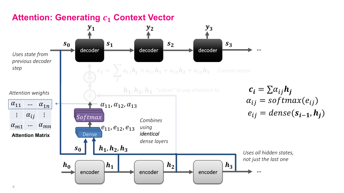
Here we walk through generating the first context vector c1. The encoder processes inputs x1 through x4, producing hidden states h1, h2, h3 at each step. To generate c1 for the first decoder step, we take the initial decoder state s0 and all encoder hidden states h1, h2, h3 and feed each pair into the same dense layer. This produces energy scores e11, e12, e13. These go through softmax to produce attention weights alpha_11, alpha_12, alpha_13, which tell us how much to weight each encoder hidden state. The context vector c1 is then the weighted sum: alpha_11 times h1 plus alpha_12 times h2 plus alpha_13 times h3. The encoder hidden states h1, h2, h3 are the "values" we pay attention to — the attention weights determine how much of each value to include. Notice the architecture uses all hidden states from the encoder, not just the last one, which is the key improvement over the basic encoder-decoder approach.

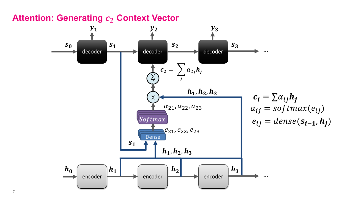
Now we generate the second context vector c2. The process is identical to c1, but this time we use the decoder state s1 instead of s0. The dense layer takes s1 paired with each encoder hidden state h1, h2, h3 to produce energy scores e21, e22, e23. Softmax converts these to attention weights alpha_21, alpha_22, alpha_23. The context vector c2 is then the weighted sum of h1, h2, h3 using these new weights. The critical point is that because s1 is different from s0 — it encodes what happened during the first decoding step — the attention weights will be different too. The model might now attend more heavily to a different part of the input. This is exactly the benefit: each decoding step gets its own tailored context vector that focuses on the most relevant encoder states for that particular output position.

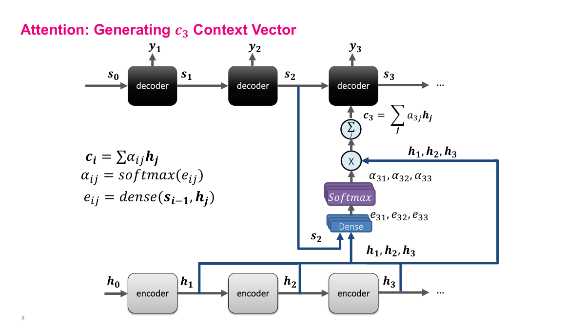
This slide shows the complete attention mechanism for generating context vector c3. The context vector ci is a weighted sum of the encoder hidden states: ci equals the sum of alpha_ij times hj. The H vectors — h1, h2, h3 — come from the encoder LSTM's hidden states at each time step. Each alpha is a scalar weight, and together they determine how much each encoder hidden state contributes to the context for a given decoder step. The architecture feeds the current decoder state s2 and all encoder hidden states h1, h2, h3 into a dense layer, which produces energy scores e31, e32, e33. These scores pass through a softmax to produce the alpha weights, which sum to one. The alphas are then multiplied element-wise with the H vectors and summed to produce c3, the context vector fed into the third decoder stage. This is the core computation of the attention mechanism — everything else is just figuring out how to compute good alpha values.

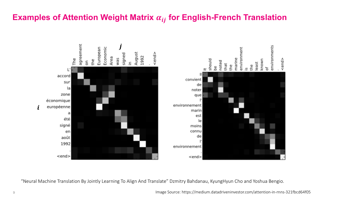
This visualization from the Bahdanau et al. paper shows what the attention weight matrix alpha_ij actually looks like for English-French translation. Each row corresponds to a French output token, and each column to an English input token. White indicates high attention weight (close to one), black indicates low weight (close to zero). Along the diagonal you can see strong correspondence — most words translate roughly one-to-one, so the model pays attention to the corresponding position. The interesting case is 'European Economic Area' which maps to 'zone économique européenne' — the word order is reversed in French. Here the attention mechanism shows its value: instead of just following the diagonal, the model learns to attend to the correct English words regardless of position. This gives interpretability — you can actually see what the model is doing. For more distant language pairs, you would expect an even less diagonal attention matrix, reflecting greater structural differences between the languages.

This is a review slide for the attention section, posing three key questions. First: what is the limitation of the basic encoder-decoder RNN architecture? The answer is the fixed-length context vector — compressing a variable-length input sequence into one fixed-size vector creates an information bottleneck, especially for long sequences. Even if you could pack all that information in, decoding it is also extremely challenging. Second: what is the attention mechanism and how does it help? Instead of passing a single vector from encoder to decoder, we use all encoder hidden states and compute a weighted sum for each decoder step. The attention mechanism decides which hidden states matter most at each step. Third: what is the intuition behind the attention weight matrix? It tells us which input tokens are most relevant for generating each output token — essentially, which parts of the input the model is paying attention to at each decoding step.

This is the section divider for self-attention. We are transitioning from the encoder-decoder attention mechanism we just covered to self-attention, which is the key innovation behind Transformers. The questions we will address include: What is self-attention? What are its inputs and outputs? Why is self-attention better than alternatives like RNNs and feedforward networks? How do parameters, compute, and memory scale as sequence length grows? What is multi-head attention? And what is positional encoding and why do we need it? The encoder-decoder attention mechanism had two nice properties — it lets the network focus attention on relevant inputs and uses parameter sharing to efficiently handle long sequences. But RNNs are slow because they process sequentially, and feedforward networks require too many parameters. The central question motivating self-attention is: can we efficiently handle long sequences without using RNNs at all?

This questions slide lays out the key topics for the self-attention section. Six questions guide our exploration: What is self-attention? What are the inputs and outputs of self-attention? Why is self-attention better than alternatives? How fast do parameters, compute, and memory grow as sequence length grows? What is multi-head attention? And what is positional encoding and why do we need it? These questions build on the attention mechanism we just covered. The core challenge is that while encoder-decoder attention works well, the underlying RNN architecture is slow — you must process tokens sequentially, creating long computational graphs with exploding and vanishing gradient problems. Feedforward networks avoid the sequential bottleneck but are parameter-inefficient, scaling as O(inputs times outputs). Self-attention will give us the benefits of attention — focused, weighted combinations of inputs — without the sequential processing constraint of RNNs.

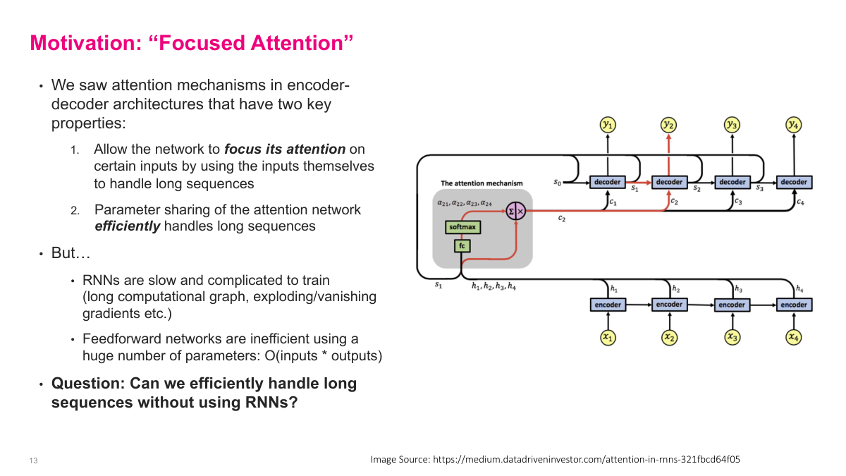
This slide motivates the move from encoder-decoder attention to self-attention. The attention mechanism in encoder-decoder architectures has two key properties. First, it allows the network to focus its attention on certain inputs by using the inputs themselves, which helps handle long sequences. Second, parameter sharing in the attention network means it efficiently handles variable-length sequences — no matter how long the input, we just add one shared weight matrix. But there are significant downsides. RNNs are slow and complicated to train because of long computational graphs and exploding or vanishing gradients. Feedforward networks are parameter-inefficient with O(inputs times outputs) parameters. This raises the central question: can we efficiently handle long sequences without using RNNs? The answer is yes — through self-attention, which was quite a breakthrough. Self-attention will let us keep the benefits of attention-based weighted combinations while eliminating the sequential processing bottleneck entirely.

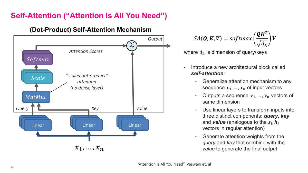
Self-attention introduces a new architectural block that generalizes the attention mechanism to any sequence of input vectors x1 through xn, outputting a sequence y1 through yn of the same dimension. The key idea from the "Attention Is All You Need" paper is to use scaled dot-product attention instead of the additive dense-layer attention from the encoder-decoder approach. Each input is transformed through three separate linear layers to produce query, key, and value vectors — analogous to the decoder state s_i and encoder hidden states h_i in regular attention. The formula is SA(Q, K, V) equals softmax of QK^T divided by the square root of dk, multiplied by V, where dk is the dimension of the query and key vectors. The scaling factor prevents dot products from becoming too large, which would push softmax into regions with tiny gradients. Attention weights are generated from the query-key interaction, and those weights determine how to combine the values to produce the final output. This replaces both the RNN and the dense-layer computation from the encoder-decoder architecture.

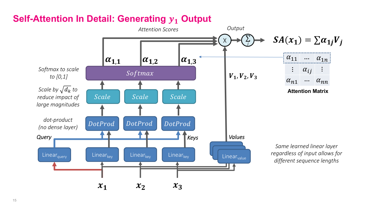
This slide shows self-attention in detail, specifically how to generate the output y1. Starting from input vectors x1, x2, x3, each input is passed through three separate linear layers to produce queries, keys, and values. The query comes from the position we are computing output for, while keys come from all positions. We compute dot products between the query and each key, scale by the square root of dk to reduce the impact of large magnitudes, then apply softmax to get attention scores alpha_1,1, alpha_1,2, and alpha_1,3 that sum to one. These alphas multiply the corresponding value vectors V1, V2, V3, and the weighted sum gives us SA(x1) — the self-attention output for position one. The full attention matrix has entries alpha_ij for all positions. Crucially, the same learned linear layers are used regardless of input sequence length, which allows self-attention to handle variable-length sequences. This replaces both the RNN and the dense-layer attention computation from the encoder-decoder architecture.

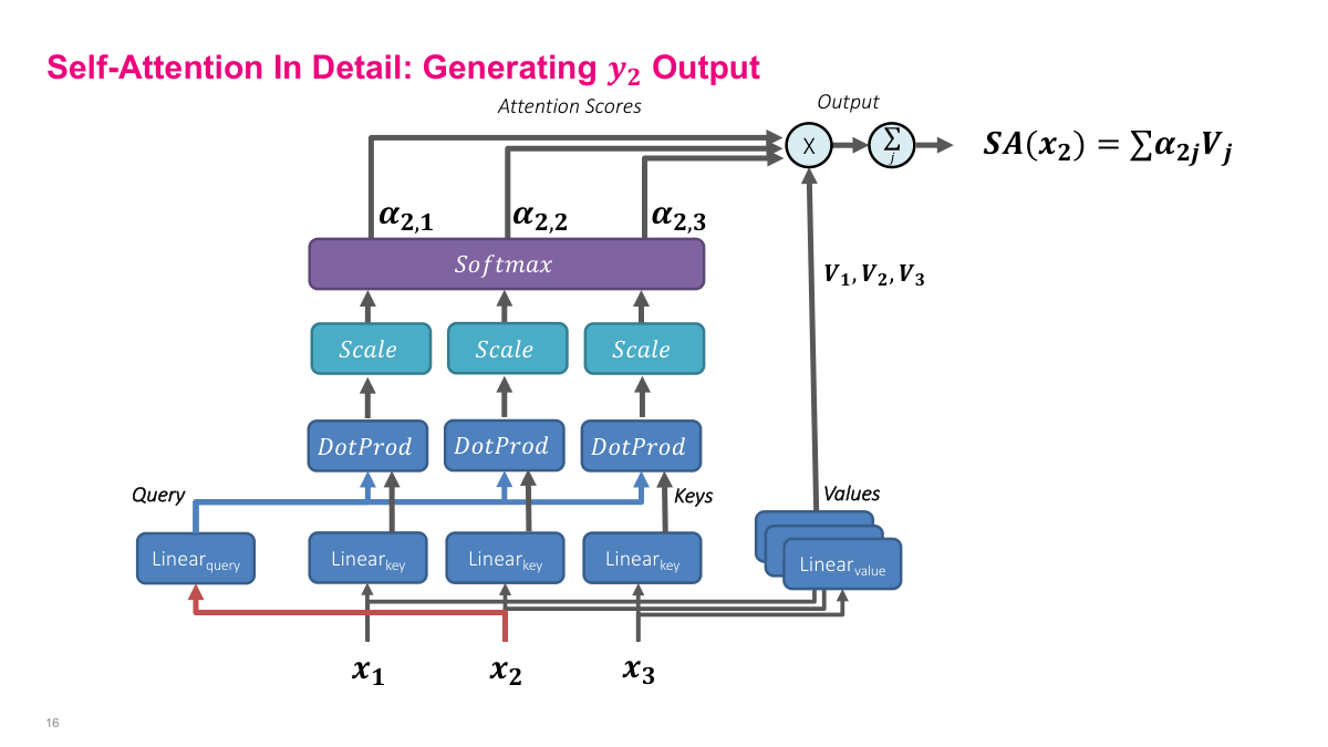
This slide shows how self-attention generates the output y2 for the second position. The process mirrors y1 but with x2 as the query source. Input x2 passes through the query linear layer to produce the query vector, while all inputs x1, x2, x3 pass through the key linear layers to produce keys. The dot product between the query from x2 and each key produces attention scores. These are scaled by the square root of dk and passed through softmax to produce attention weights alpha_2,1, alpha_2,2, alpha_2,3. These weights multiply the value vectors V1, V2, V3 and sum to produce SA(x2) — the self-attention output for position two. The key insight is that the same linear layers are shared across all positions — only the query source changes. The query asks "what should I attend to?", the keys answer "here's what I contain," and the values provide the actual content to aggregate. This parameter sharing is what makes self-attention efficient regardless of sequence length.

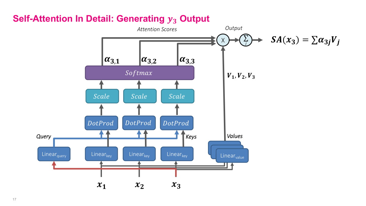
This slide completes the self-attention walkthrough by showing how y3 is generated for the third position. Now x3 is the query source — it passes through the query linear layer while all inputs pass through key and value layers. The dot products between the x3 query and all keys produce attention scores, which after scaling and softmax give alpha_3,1, alpha_3,2, alpha_3,3. These weights combine the value vectors to produce SA(x3). After computing all three outputs, we have the full attention matrix with entries alpha_ij for all position pairs. Each row sums to one and represents how much each position attends to every other position. The entire computation can be parallelized — unlike RNNs, all positions can be computed simultaneously since there are no sequential dependencies. This is the fundamental advantage of self-attention over recurrent architectures and why Transformers train so much faster on modern GPU hardware.

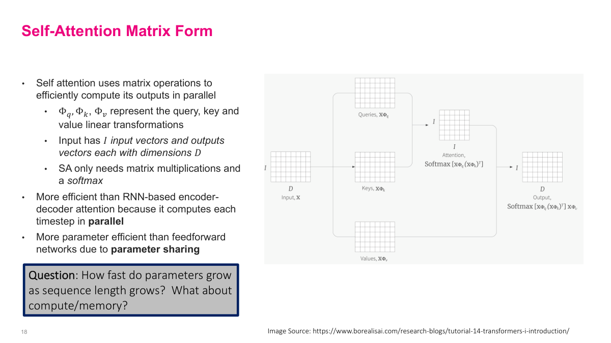
Self-attention can be expressed entirely as matrix operations, which is key to its computational efficiency. The input matrix X has I input vectors of dimension D. Three learned weight matrices Phi_q, Phi_k, and Phi_v transform X into queries, keys, and values respectively. The attention computation is then just matrix multiplications and a softmax: the output equals softmax of XPhi_q times (XPhi_k)^T, multiplied by X*Phi_v. This is more efficient than RNN-based encoder-decoder attention because all timesteps are computed in parallel — there are no sequential dependencies. It is also more parameter efficient than feedforward networks due to parameter sharing — the same weight matrices are applied regardless of sequence length. The slide raises the important question: how fast do parameters grow as sequence length increases? For self-attention, parameters are fixed (just the three weight matrices), but compute and memory grow quadratically with sequence length due to the I-by-I attention matrix. This quadratic scaling is the main limitation of self-attention.

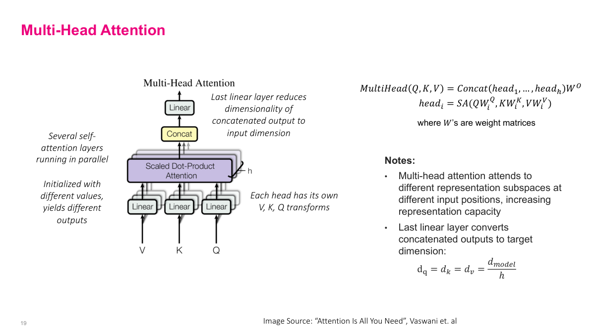
Multi-head attention runs several self-attention layers in parallel, each with its own learned weight matrices. Each head_i computes SA(QW_i^Q, KW_i^K, VW_i^V) independently, and the outputs are concatenated and projected through a final linear layer: MultiHead(Q,K,V) = Concat(head_1,...,head_h) W^O. Each head attends to different representation subspaces at different input positions, increasing the model's representation capacity. Since each head has its own V, K, Q transformations initialized with different values, they learn to capture different types of relationships — one head might attend to syntactic structure while another focuses on semantic similarity. To keep the total computation comparable to single-head attention, the dimension of each head is reduced: d_q = d_k = d_v = d_model / h. The final linear layer converts the concatenated h-head outputs back to the target dimension. This is analogous to how multiple convolutional filters capture different features in CNNs.

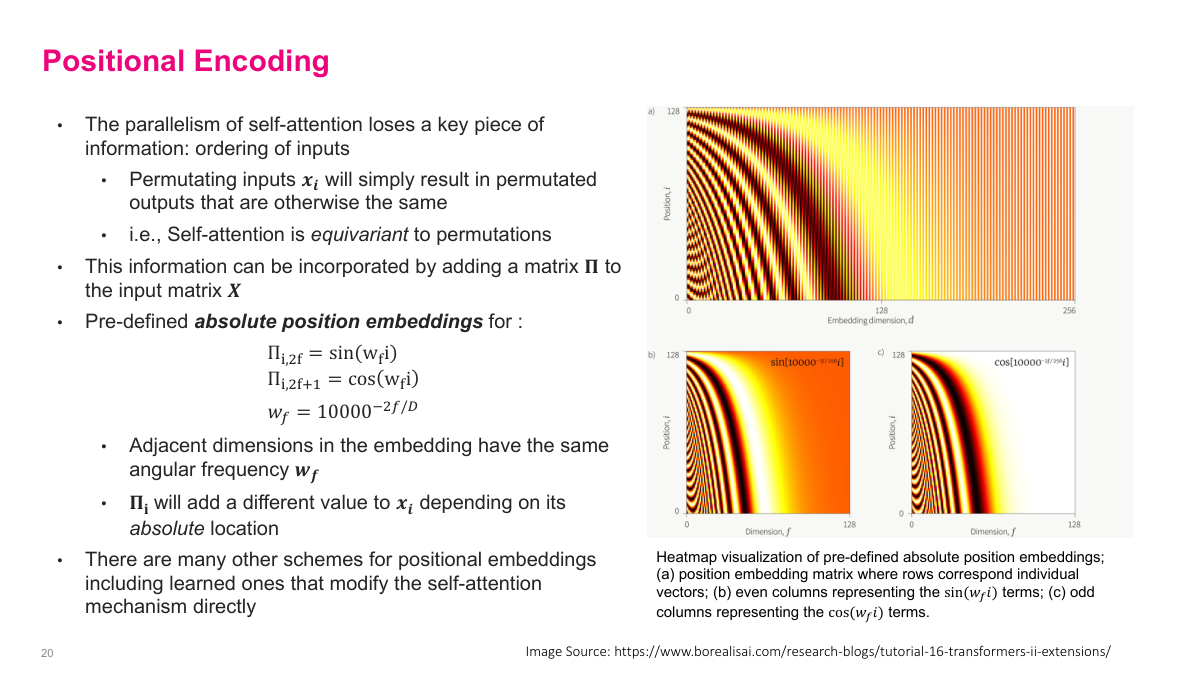
A fundamental limitation of self-attention is that it is permutation-equivariant — permuting the input vectors will simply result in permuted outputs with otherwise the same values. This means self-attention has no notion of ordering, which is clearly a problem for sequential data like language. Positional encoding solves this by adding a matrix B to the input matrix X, where each row of B encodes the position of that token. The pre-defined absolute positional encoding uses sinusoidal functions: the even dimensions use sine and odd dimensions use cosine, each with a different angular frequency w_k = 1/10000^(2k/d). Adjacent dimensions in the embedding have the same angular frequency, and each pair has a different value to uniquely encode position. The heatmap visualization shows how different positions and dimensions produce distinct patterns. There are many other schemes for positional encoding, including learned encodings and relative position approaches that modify the self-attention mechanism directly.

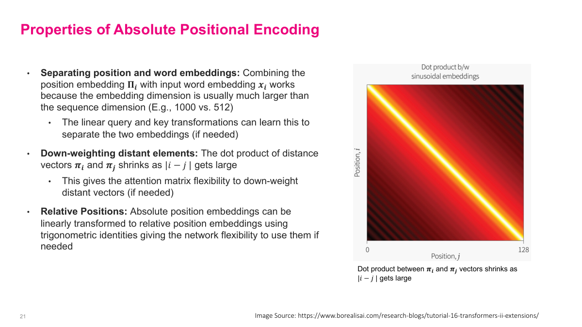
Absolute positional encoding has several important properties. First, position and word embeddings are combined by separating them — the position embedding B_i is combined with the input word embedding x_i. Because the embedding dimension is usually much larger than what position encoding needs, the linear query and key transformations can learn to separate positional from semantic information. Second, the dot product between distant elements naturally shrinks as the distance between positions grows — the positional encoding vectors become less similar as positions get farther apart. This gives the attention mechanism a built-in bias toward attending to nearby tokens, which is often desirable. Third, absolute positional encodings can be linearly transformed to relative position encodings using trigonometric identities, giving the network flexibility to use them in either way. The right-side visualization shows how the dot product between position vectors decays with distance, confirming the distance-dependent shrinkage property.

This review slide covers the self-attention section with six key questions. Self-attention is a mechanism that computes weighted combinations of input vectors using queries, keys, and values derived from the inputs themselves. Its inputs are a sequence of vectors x1 through xn, and its outputs are a sequence y1 through yn of the same dimension. Self-attention is better than RNNs because it computes all positions in parallel rather than sequentially, and better than feedforward networks because parameter sharing keeps the parameter count fixed regardless of sequence length. Parameters do not grow with sequence length — only the three weight matrices matter — but compute and memory grow quadratically due to the n-by-n attention matrix. Multi-head attention runs multiple self-attention heads in parallel with different learned projections, capturing different types of relationships. Positional encoding adds position information to inputs since self-attention is inherently permutation-equivariant and has no built-in notion of order.

Now we move into the Transformer architecture itself — the culmination of attention and self-attention concepts we've been building up. We've covered how attention allows decoders to selectively focus on encoder hidden states, and how self-attention removes the need for RNNs by computing all positions in parallel. The Transformer puts these ideas together into a complete architecture that has become the foundation of modern language models. In this section we'll cover the Transformer block and its components, the difference between encoder and decoder variants, specific architectures like BERT and GPT, and how to train and generate text with these models. This is where everything comes together — the Transformer architecture is what powers large language models today, from GPT to BERT and beyond.

This questions slide outlines six key topics for the Transformers section. First: what is the transformer block — the basic building unit that gets stacked to form deep models? Second: what is the difference between a transformer encoder and decoder block — encoder blocks use bidirectional self-attention while decoder blocks use masked (causal) self-attention? Third and fourth: describe the BERT and GPT architectures and their applications — BERT is an encoder-only model for understanding tasks, while GPT is a decoder-only model for text generation. Fifth: how do you train a GPT architecture — using autoregressive language modeling where the model predicts the next token? Sixth: how do you generate text using a GPT architecture — by sampling tokens one at a time from the model's predicted probability distribution? These questions will guide us through the practical side of Transformers.

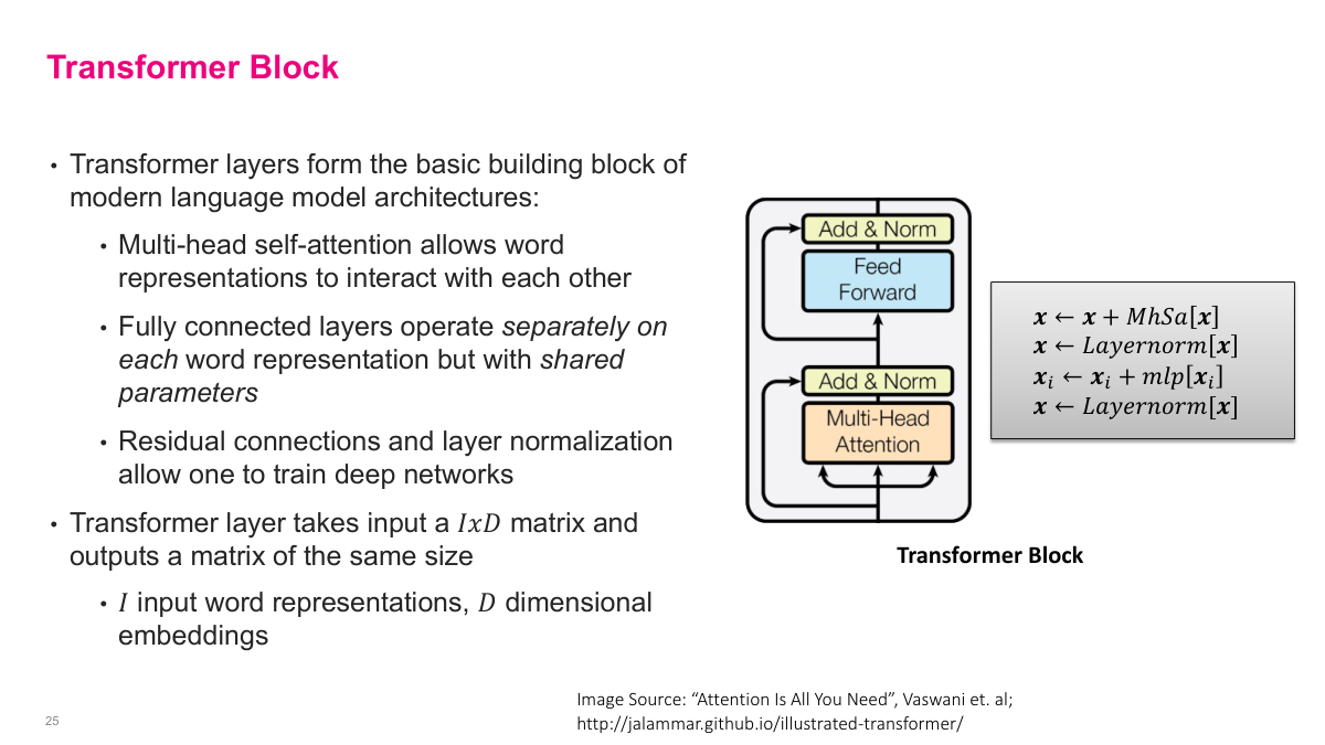
The answer is yes — we can do better with self-attention, and it was quite a breakthrough. The Transformer block is the basic building block of modern language model architectures. It has several key components working together. First, multi-head self-attention allows word representations to interact with each other — this is where each token can attend to every other token in the sequence. Second, fully connected layers operate separately on each word representation but with shared parameters, keeping the model efficient. Third, residual connections and layer normalization allow us to train very deep networks without degradation. The Transformer layer takes an input matrix of size I by D — where I is the number of input word representations and D is the embedding dimension — and outputs a matrix of the same size. This is elegant: you can stack these blocks on top of each other repeatedly. The computation flows upward through multi-head attention, then add-and-normalize, then a feedforward layer, then another add-and-normalize. Each step refines the representations while maintaining the same dimensions.

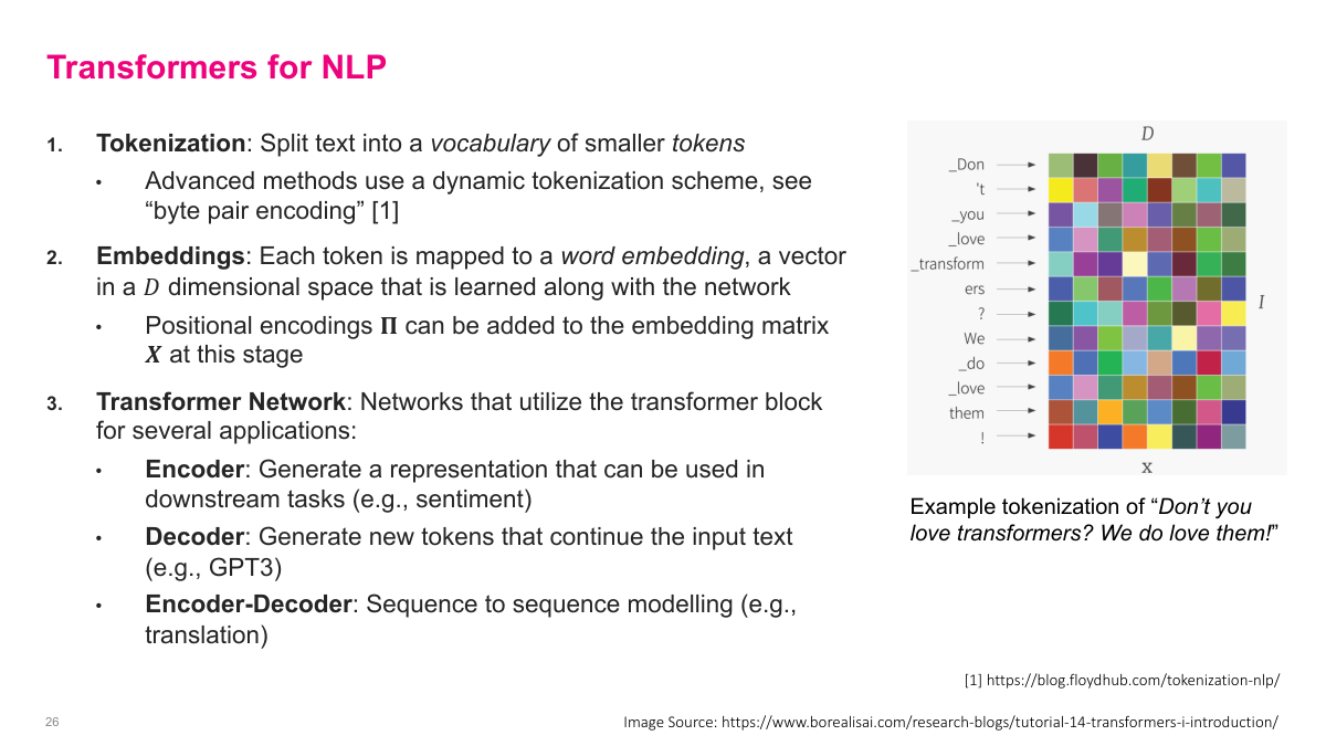
To use Transformers for NLP, we need three key ingredients. First, tokenization: we split text into a vocabulary of smaller tokens. Advanced methods use dynamic tokenization schemes like byte pair encoding, which can handle any text by breaking unfamiliar words into subword pieces. Second, embeddings: each token is mapped to a word embedding, a vector in a D-dimensional space that's learned along with the network. Positional encodings can be added to the embedding matrix at this stage to give the model information about token order. Third, the Transformer network itself, which stacks transformer blocks for different applications. An encoder generates a representation useful for downstream tasks like sentiment analysis. A decoder generates new tokens that continue the input text — this is what GPT-3 does. An encoder-decoder combines both for sequence-to-sequence tasks like translation. The example on the slide shows how a sentence gets tokenized into pieces, with each token becoming a row in the I-by-D embedding matrix X that feeds into the Transformer blocks.

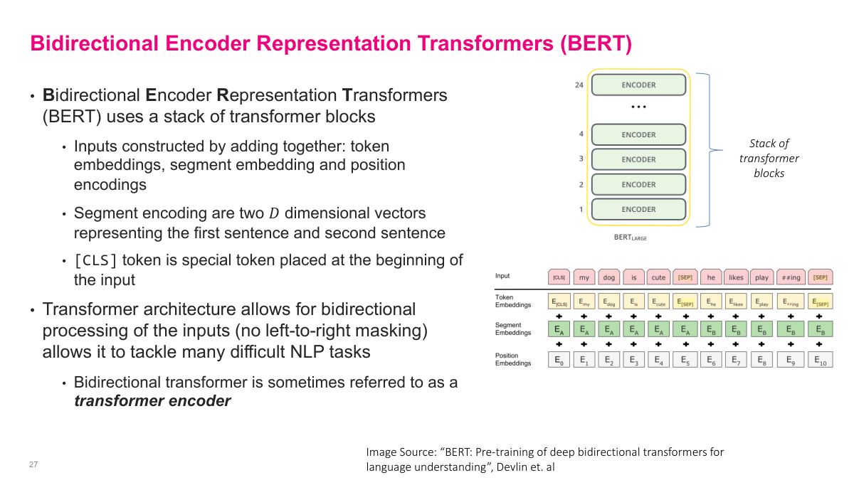
BERT — Bidirectional Encoder Representation Transformers — uses a stack of transformer encoder blocks. BERT-Large stacks 24 encoder blocks on top of each other. The inputs are constructed by adding together three types of embeddings: token embeddings for the actual words, segment embeddings that distinguish between a first and second sentence, and position encodings that capture where each token sits in the sequence. The segment encodings are just two D-dimensional vectors representing sentence A and sentence B. A special CLS token is placed at the beginning of the input, and a SEP token separates the two sentences. The critical feature of BERT is that the transformer architecture allows bidirectional processing of the inputs — there's no left-to-right masking. Every token can attend to every other token in both directions. This makes it powerful for many NLP tasks because it captures full context. A bidirectional transformer is sometimes referred to as a transformer encoder, as opposed to the decoder architecture used in models like GPT.

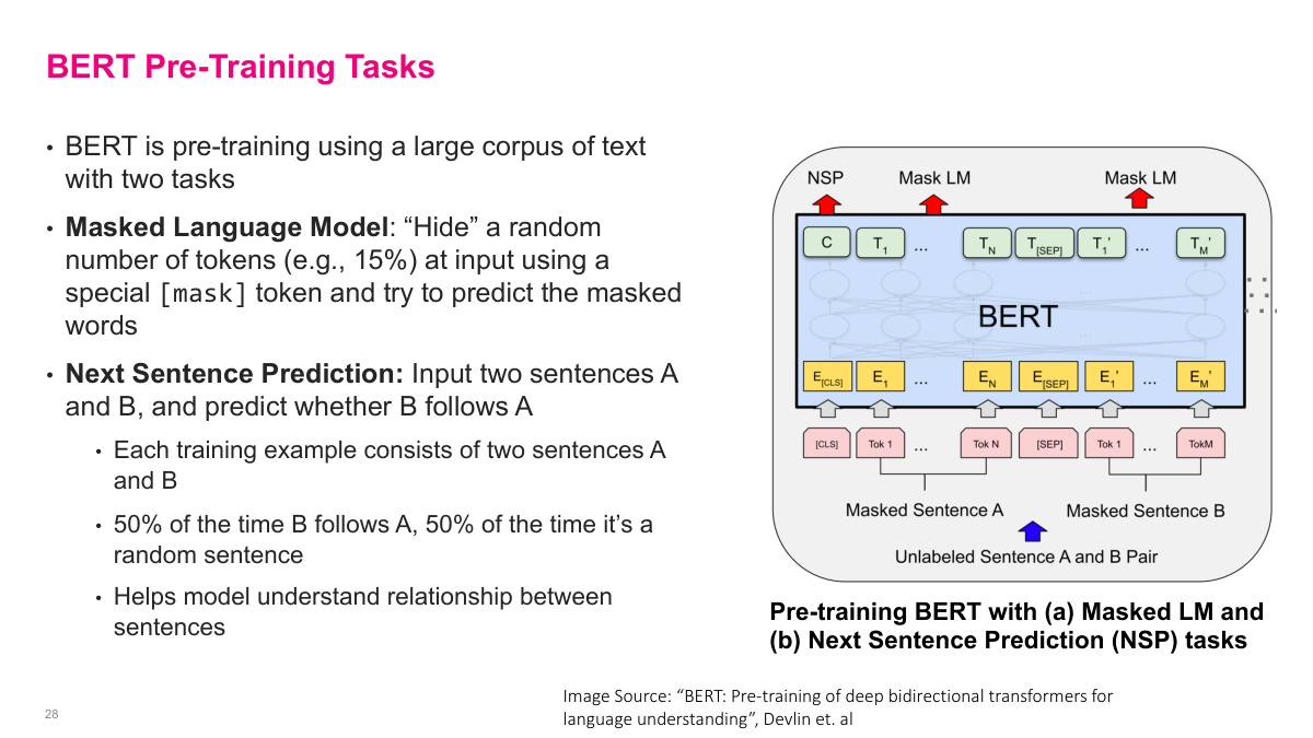
BERT is pre-trained on a large corpus of text using two clever self-supervised tasks. The first is the Masked Language Model: randomly hide about 15% of the input tokens by replacing them with a special mask token, then train the model to predict those masked words. This forces BERT to build deep contextual understanding because it needs surrounding context from both directions to figure out what's missing. The second task is Next Sentence Prediction: input two sentences A and B, and predict whether B actually follows A in the original text. During training, 50% of the time B genuinely follows A, and 50% of the time it's a random sentence. This helps the model understand relationships between sentences, which is important for tasks like question answering and natural language inference. Together, these two pre-training objectives give BERT a rich understanding of language structure and meaning, all learned from unlabeled text — no manual annotation required.

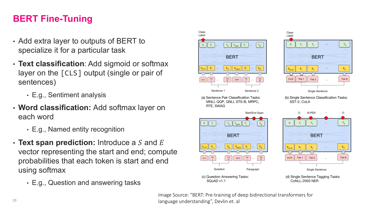
Once BERT is pre-trained, fine-tuning it for specific tasks is straightforward — you just add an extra layer on top of the pre-trained model. For text classification tasks like sentiment analysis, you add a sigmoid or softmax layer on the CLS token output to classify single sentences or sentence pairs. For word classification tasks like named entity recognition, you add a softmax layer on each word's output to classify every token individually. For text span prediction tasks like question answering, you introduce a start vector and end vector, then compute probabilities that each token is the start or end of the answer span. The beauty of this approach is that the massive pre-trained BERT model has already learned rich language representations. Fine-tuning just adjusts those representations slightly for your specific task, requiring far less labeled data and training time than building a model from scratch. This pre-train-then-fine-tune paradigm became the dominant approach in NLP after BERT's introduction.

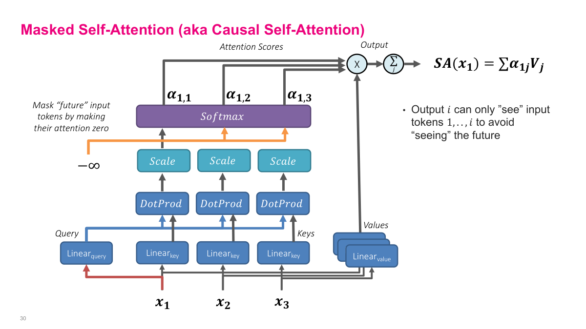
Masked self-attention, also called causal self-attention, adds one critical modification to the self-attention mechanism we just discussed. The diagram here shows the same query, key, value structure — each input token X gets transformed through separate linear layers to produce queries, keys, and values. We compute dot products between queries and keys, scale them, and apply softmax to get attention weights. But here's the key difference: we mask out future tokens by setting their attention scores to negative infinity before the softmax. This forces the softmax output to zero for those positions. The result is that output i can only "see" input tokens 1 through i — it cannot look ahead at future tokens. This is essential for autoregressive language modeling, where we're predicting the next word based only on previous words. If the model could see future tokens during training, it would be cheating. The masking ensures the model learns to generate text left-to-right, one token at a time, which is exactly what we need at inference time when future tokens don't exist yet.

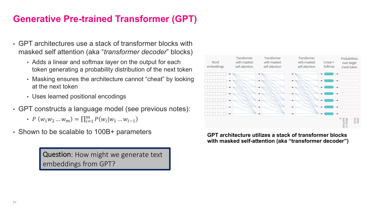
GPT — the Generative Pre-trained Transformer — takes the self-attention mechanism we've been building up and turns it into a powerful language model. The architecture uses a stack of transformer blocks, each containing masked self-attention. These are called "transformer decoder" blocks because they use that causal masking we just discussed. On top of the stack, GPT adds a linear layer followed by a softmax to produce a probability distribution over the next token. The masking is what prevents the architecture from cheating by looking at future tokens. GPT also uses learned positional encodings rather than the sinusoidal ones we discussed earlier. Mathematically, GPT constructs a language model: the probability of a sequence of words equals the product of conditional probabilities P(w_i | w_1, ..., w_{i-1}). This factorization is exactly what the masked self-attention enables. The architecture has been shown to scale to over 100 billion parameters. An interesting question the slide poses: how might we generate text embeddings from GPT? That's a useful capability beyond just text generation.

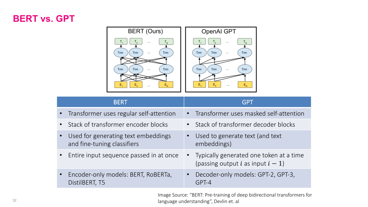
This slide draws the key distinction between BERT and GPT — two foundational transformer architectures that take opposite approaches. BERT uses regular, bidirectional self-attention in a stack of transformer encoder blocks. Every token can attend to every other token, both before and after it. This makes BERT excellent for generating contextualized word embeddings and fine-tuning classifiers, but it means you can't use it directly for text generation. GPT uses masked self-attention in transformer decoder blocks, so each token only attends to previous tokens. This autoregressive structure is designed for generating text one token at a time. BERT processes the entire input sequence at once, while GPT generates tokens sequentially, feeding each output back as input. The encoder-only family includes BERT, RoBERTa, DistilBERT, and T5. The decoder-only family includes GPT-2, GPT-3, and GPT-4. Both architectures build on the same self-attention foundation we've been developing, but the presence or absence of masking fundamentally changes what tasks they're suited for.

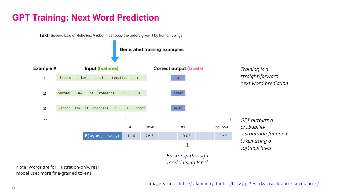
GPT training is remarkably straightforward — it's simply next word prediction. Take a sentence like "Second Law of Robotics: A robot must obey the orders given it by human beings." We generate training examples by sliding a window through the text. Example 1: input is "Second law of robotics :" and the correct output label is "a." Example 2: the input grows to include "a" and the label is "robot." Example 3: input includes "a robot" and the label is "must." And so on. For each example, GPT outputs a probability distribution over the entire vocabulary using a softmax layer. The word "must" might get probability 0.02 while other words get much smaller values. We then backpropagate through the model using the correct label to update parameters. Note that in practice, the model uses more fine-grained tokens rather than whole words — this is just for illustration. The beauty of this approach is that training data is essentially free: any text corpus provides unlimited supervised examples without human labeling.

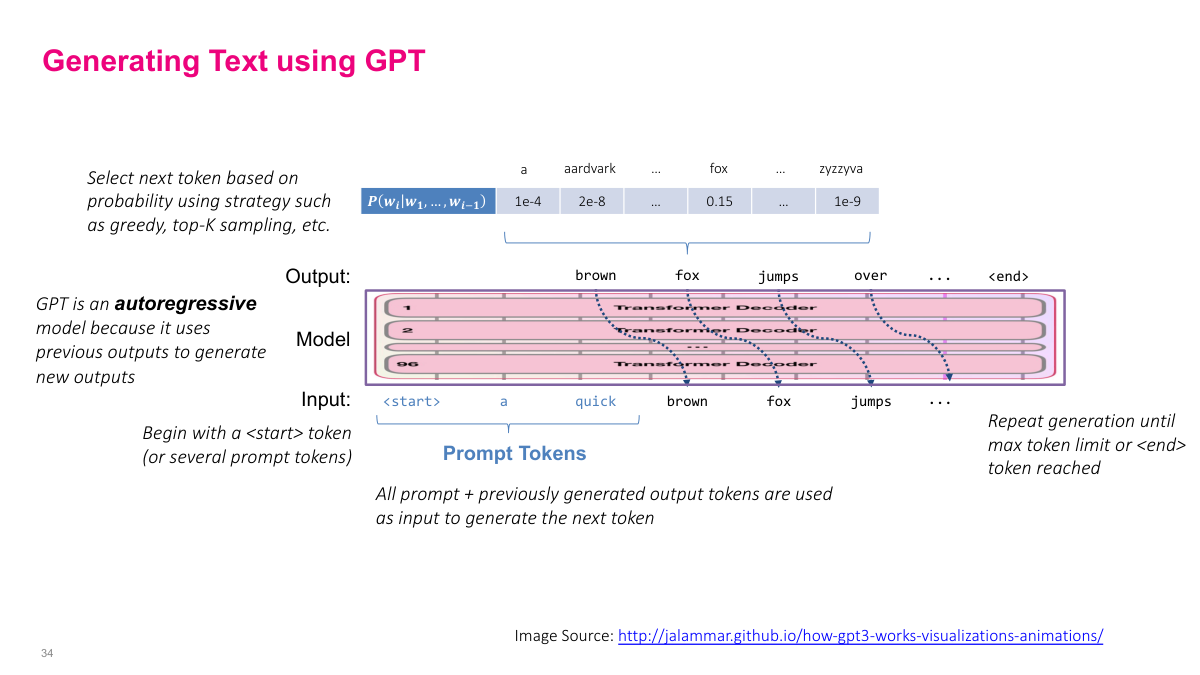
Text generation with GPT is an autoregressive process. We start with a prompt — a start token or several prompt tokens — and feed them into the model. The model outputs a probability distribution over the entire vocabulary for the next token. We select the next token based on this distribution using a strategy like greedy decoding, top-K sampling, or other approaches. That selected token then gets appended to the input, and we feed the entire sequence — prompt plus all previously generated tokens — back through the model to generate the next token. This process repeats: each step, the full sequence of prompt plus generated tokens goes through the stack of transformer decoder blocks, producing the next token's probability distribution. We keep generating until we hit a maximum token limit or produce an end token. This is why GPT is called an autoregressive model — it uses its own previous outputs to generate new outputs. The masked self-attention ensures that at each position, the model only attends to tokens that came before it, which is exactly this left-to-right generation pattern.

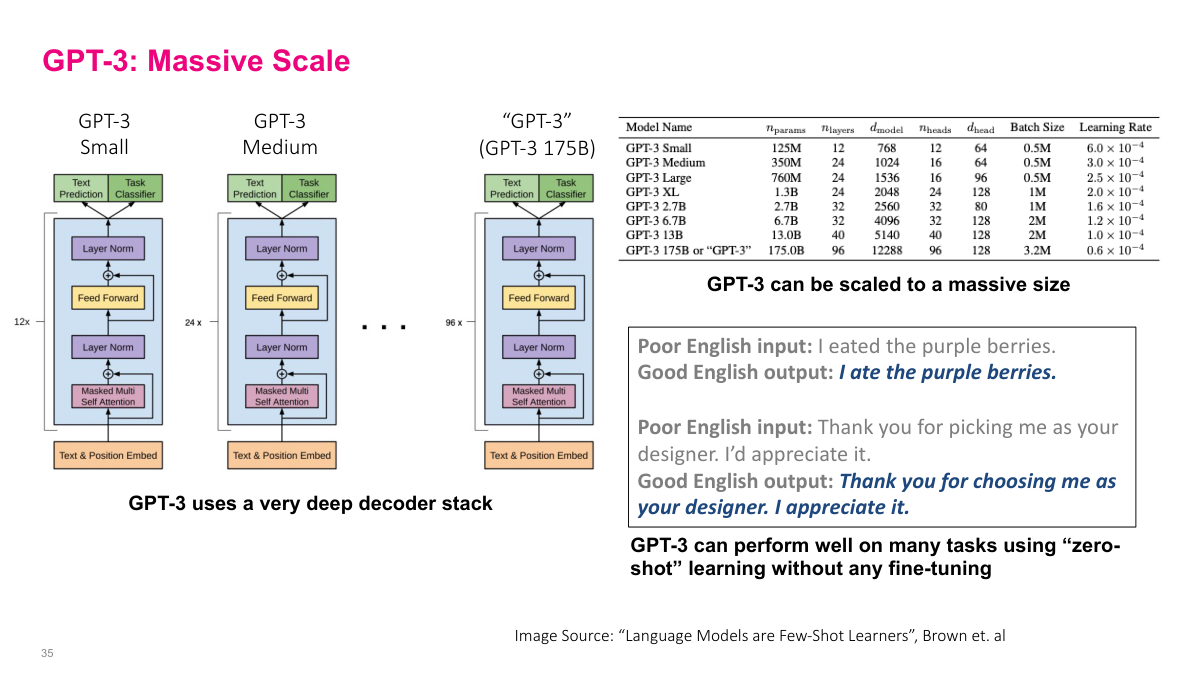
GPT-3 demonstrates the power of scaling transformer decoder architectures massively. The slide shows several model sizes — from GPT-3 Small at 125 million parameters up to the full GPT-3 at 175 billion parameters. As models get larger, they use more layers, wider hidden dimensions, more attention heads, and larger batch sizes. GPT-3 Small has 12 layers and 12 attention heads, while the full 175B model uses 96 layers and 96 heads. The architecture diagram shows the same basic structure repeated — text and position embeddings feeding into stacked blocks of masked self-attention, layer normalization, and feed-forward layers. It's just a very deep decoder stack. What's remarkable is that GPT-3 can perform well on many tasks using zero-shot learning — no fine-tuning at all. The examples show it correcting grammar from "I eated the purple berries" to "I ate the purple berries" and improving writing style, all without task-specific training. This emergent capability from pure scale was a significant finding.

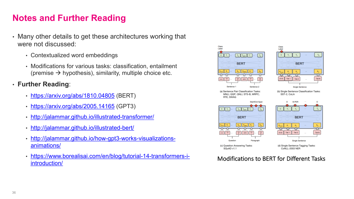
There are many details we haven't covered that go into making these architectures work in practice — contextualized word embeddings, modifications for different tasks like classification, entailment, similarity, and multiple choice. The slide shows how BERT can be adapted for various downstream tasks: sentence pair classification for tasks like MNLI and MRPC, single sentence classification for SST-2 and CoLA, question answering for SQuAD, and sequence tagging for named entity recognition. Each task requires slightly different input formatting and output heads, but the core pretrained BERT model stays the same. For further reading, the key papers are the original BERT paper by Devlin et al. and the GPT-3 paper "Language Models are Few-Shot Learners" by Brown et al. Jay Alammar's illustrated guides to transformers, BERT, and GPT-3 are excellent visual resources for building intuition. The Borealis AI tutorial on transformers is another solid introduction to these concepts.

This final review covers the Transformers section with six key questions. The transformer block is the basic building unit: it combines multi-head self-attention, feedforward layers, residual connections, and layer normalization, taking an I-by-D matrix as input and outputting the same dimensions. The difference between encoder and decoder blocks is masking: encoder blocks use bidirectional self-attention where every token attends to every other token, while decoder blocks use masked (causal) self-attention where tokens can only attend to previous positions. BERT is an encoder-only architecture that stacks transformer encoder blocks, pre-trained with masked language modeling and next sentence prediction, then fine-tuned for classification, question answering, and other understanding tasks. GPT is a decoder-only architecture using masked self-attention, designed for text generation. GPT is trained via next word prediction — given a sequence of tokens, predict the next one — using freely available text corpora. Text generation is autoregressive: start with a prompt, generate one token at a time by sampling from the predicted probability distribution, and feed each generated token back as input for the next step.