Lecture 02: Training Neural Networks

Building a neural network is surprisingly easy with modern frameworks. In the assignments, you'll use Keras, one of the higher-level Python libraries for deep learning. Using the Sequential API, you stack layers — and remember, "dense" is another name for feedforward neural network layers. Each Dense layer takes a parameter for how many neurons you want. So here we have a three-layer network with widths of two, three, and one neuron respectively. You specify the activation function for each layer, and if you omit it, you get the identity function — meaning the output can range from negative to positive infinity. Once trained, using the model is like calling a function: you pass in an input vector and get output values back. The whole thing is about five lines of code. For contrast, when I was interning, we built a handwritten digit recognizer in two or three hundred lines of C, writing all the training and backpropagation code ourselves. Now the frameworks handle all of that behind the scenes.

Back in the day, building a neural network for something as basic as handwritten digit recognition required writing hundreds of lines of C code — including all the training logic, backpropagation, and debugging. Today, you accomplish the same thing with just a couple of function calls. You call compile to set up the model configuration, and fit to actually train it. The fit step is where all the learning happens, running the training algorithms behind the scenes. The second assignment will walk you through exactly how this works. The contrast really highlights how much the tooling has evolved — what once took significant low-level programming effort is now abstracted into simple, high-level API calls.

The fit call is the training step, and all the optimization algorithms are hidden behind the scenes. But here's an important caveat: even though you won't be writing your own backpropagation algorithm, it's still critical to understand how these things work under the hood. If you treat the framework as a pure black box, you'll inevitably run into weird behavior that you can't explain. The model won't do what you want, and you'll have no idea how to debug it. Understanding the internals gives you the mental model you need to diagnose problems when they arise. This is a recurring theme throughout the course — we use high-level tools for practical work, but we study the underlying mathematics and algorithms so you can reason about what's actually happening inside the network.

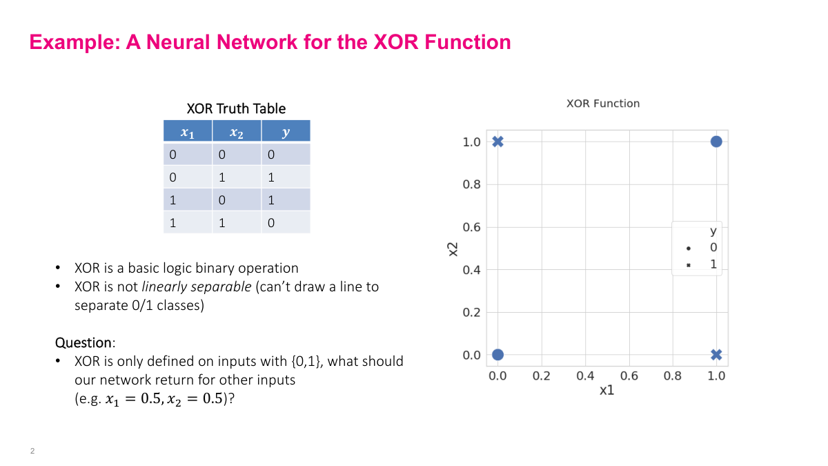
Even though frameworks handle backpropagation for you, understanding the mechanics is essential for debugging and building intuition. Now, we covered neural network terminology and architecture last time — feedforward networks, layers, activations. And as you saw in the code, adding 100 layers is trivial: just write a for loop. Making big neural networks is easy. The hard question is: these networks have millions, billions, even trillions of parameters. How do you pick the right numbers? How do you train them? That's what this lecture covers. But first, a historical example. Remember that 1960s paper claiming neural networks could never work? The argument was they couldn't learn the XOR function — a simple binary logic operation. The truth table shows: given inputs X1 and X2, the output is like OR except that (1,1) maps to 0. If you graph it, you get this pattern where the classes aren't linearly separable. It's a simple function we'd expect a neural network to learn. An interesting question arises: what should the network output at a point like (0.5, 0.5), which isn't in our training data?

What should the neural network output at (0.5, 0.5)? Should it return minus one million? That doesn't seem reasonable. The real answer is there is no right answer — we haven't defined the function at that point. We only defined values at the four corners of our truth table. Since we never told the neural network what the output should be at (0.5, 0.5), it's going to pick something on its own. It probably won't be anything extreme like minus one million, but it could be close to zero, close to one — we don't know exactly. This highlights an important property of machine learning: you give the network examples and it figures out the pattern. But the caveat is critical — if you don't provide an example for a particular input, and that input matters to you, the network will just pick something, and it probably won't be what you want. You need to supply training examples for the behaviors you care about.

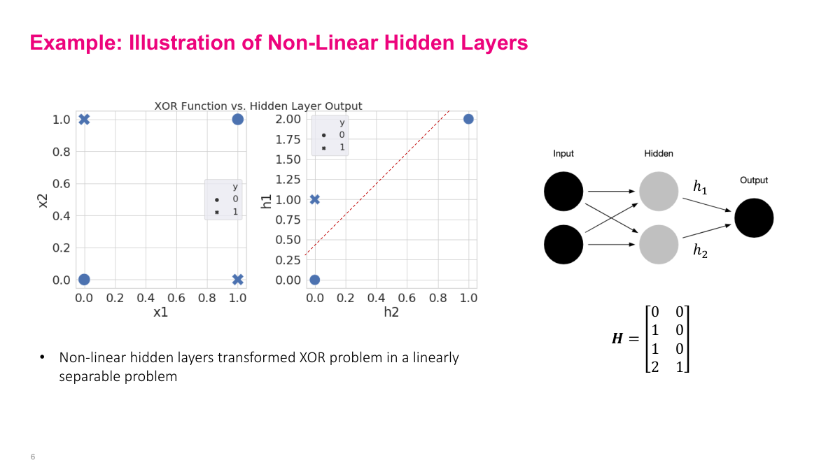
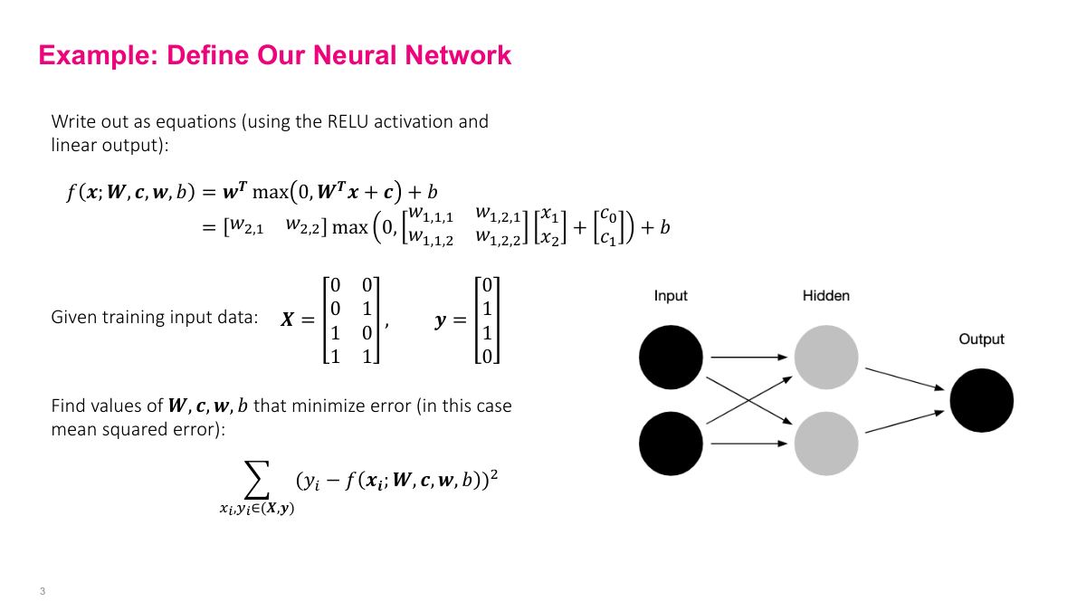
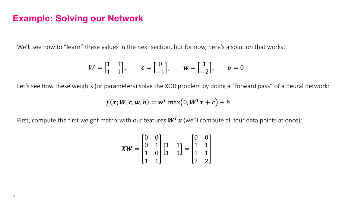
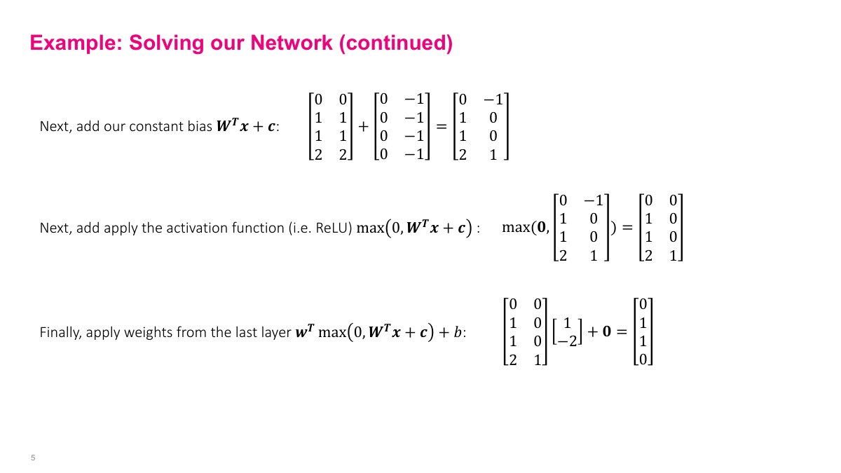
The reason that 1960s paper got it wrong is that you need more than one layer and nonlinearities to solve XOR. A single-layer network cannot do it. You need at least two layers — here we have a hidden layer with two neurons and an output layer with one neuron. The inputs X1 and X2 are just features. I've written out the math so you can follow the actual computation: propagating inputs through the network to produce outputs. I'm computing all four inputs simultaneously in batch form, because in practice you use GPUs that process hundreds of examples at once — that's how NVIDIA hardware works most efficiently. For this example, I'm giving you the parameters directly: weight matrix W is all ones, first layer biases are 0 and -1, second layer weights are 1 and -2, output bias is 0. The first computation step is multiplying inputs by the weight matrix. Then we add the bias vector — a constant added to each neuron's output. The bias is the same across all examples in the batch.

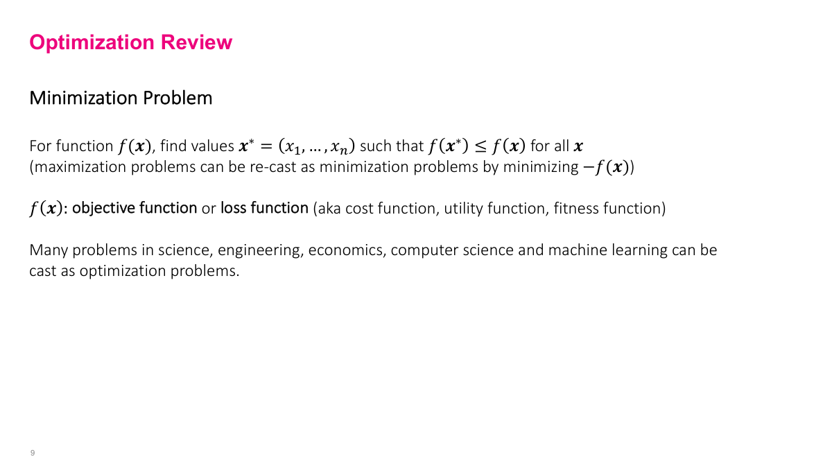
Optimization is really about minimization — find the input values that minimize some function. You can always convert a maximization problem to minimization by negating the function, so they're equivalent. In machine learning, we frame everything as minimization. The function we're minimizing could have multiple inputs, essentially a vector-valued function, and we want to find the input that gives us the smallest possible output across all possible inputs. Optimization problems appear in every discipline of science and engineering, but machine learning has its own terminology. We call this function the objective function or, more commonly, the loss function. You'll also hear terms like cost function, utility function, or fitness function in other domains, but they all capture the same idea: we have some function that measures how well or poorly our model is doing, and we want to minimize it.

The critical distinction in optimization is between convex and non-convex functions. A convex function has a simple visual test: pick any two points on the curve, draw a line segment between them, and that segment stays entirely above or on the curve. For non-convex functions, you can find two points where the line segment dips below the curve. Why does this matter so much? For convex functions, any local minimum you find is guaranteed to be the global minimum. That's a powerful property. For non-convex functions, you can get stuck in a local minimum that's far from the global optimum — you can see that red dot sitting in a local valley that clearly isn't the lowest point. We have many reliable techniques for finding local minima, but finding the absolute global minimum of a non-convex function is generally intractable. So convex functions are ideal. Among the many optimization methods available — simplex, Newton's method, coordinate descent, simulated annealing — the only one we really care about for deep learning is stochastic gradient descent and its variations.

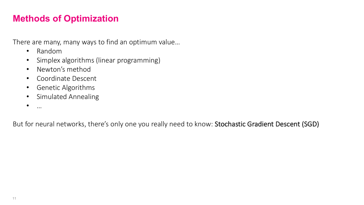
There are many methods for finding optimal values — random search, simplex algorithms for linear programming, Newton's method, coordinate descent, genetic algorithms, simulated annealing, and more. Each has its niche, but for neural networks, there's really only one you need to know: Stochastic Gradient Descent, or SGD. The reason is practical — most of these other methods either don't scale to the millions of parameters we deal with in deep learning, or they require information (like second derivatives) that's too expensive to compute. SGD is simple, scales well, and works surprisingly effectively for training neural networks.

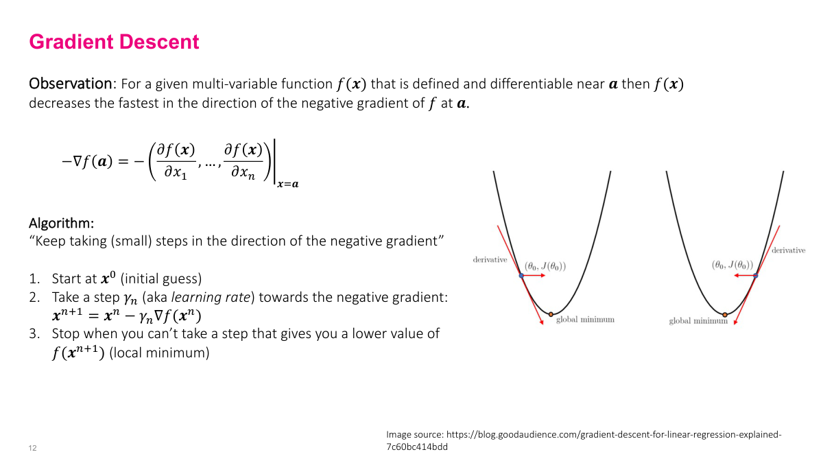
The gradient descent algorithm boils down to one rule: keep taking small steps in the direction of the negative gradient. You start with some initial guess, then iteratively update your position. The key parameter is the step size, often called gamma or the learning rate. You don't have to use the same step size at every iteration — it can vary. Under certain conditions, if you take enough steps with appropriate step sizes, you'll converge to a local minimum or get arbitrarily close to one. Let's see this in action with a concrete example. Starting at x equals 0.1, with a step size that halves each iteration, we can trace the algorithm's behavior. Initially the gradient is small because the function is relatively flat near the starting point, so the steps are small. As we move into steeper territory, the steps get bigger because the gradient is larger, even as the step size is shrinking. Near the bottom, where the function flattens out and the step size has gotten small, the algorithm settles into the minimum around negative 2.5.

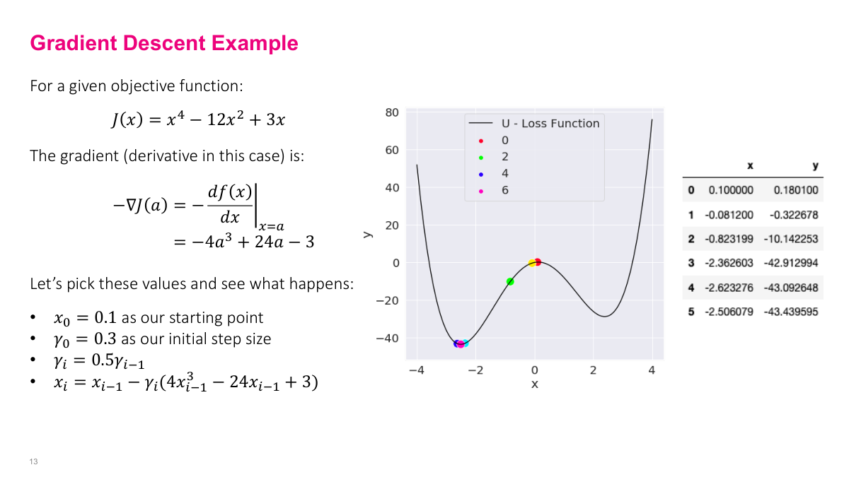
Looking at the numerical values from our gradient descent example, you can see the algorithm converging to approximately negative 2.5, which corresponds to the minimum of this function on the graph. The trajectory tells the whole story of gradient descent in practice: the algorithm navigates the landscape by following the local slope at each point. Where the function is steep, it takes larger effective steps; where it's flat, the steps are naturally smaller. Combined with the decaying step size that halves each iteration, the algorithm transitions from exploration to fine-tuning as it approaches the minimum. The key takeaway is how simple this really is — at each iteration, we just compute the gradient, multiply by our step size, and subtract from our current position. That's the entire algorithm. Despite this simplicity, gradient descent is remarkably effective and forms the backbone of all deep learning optimization.

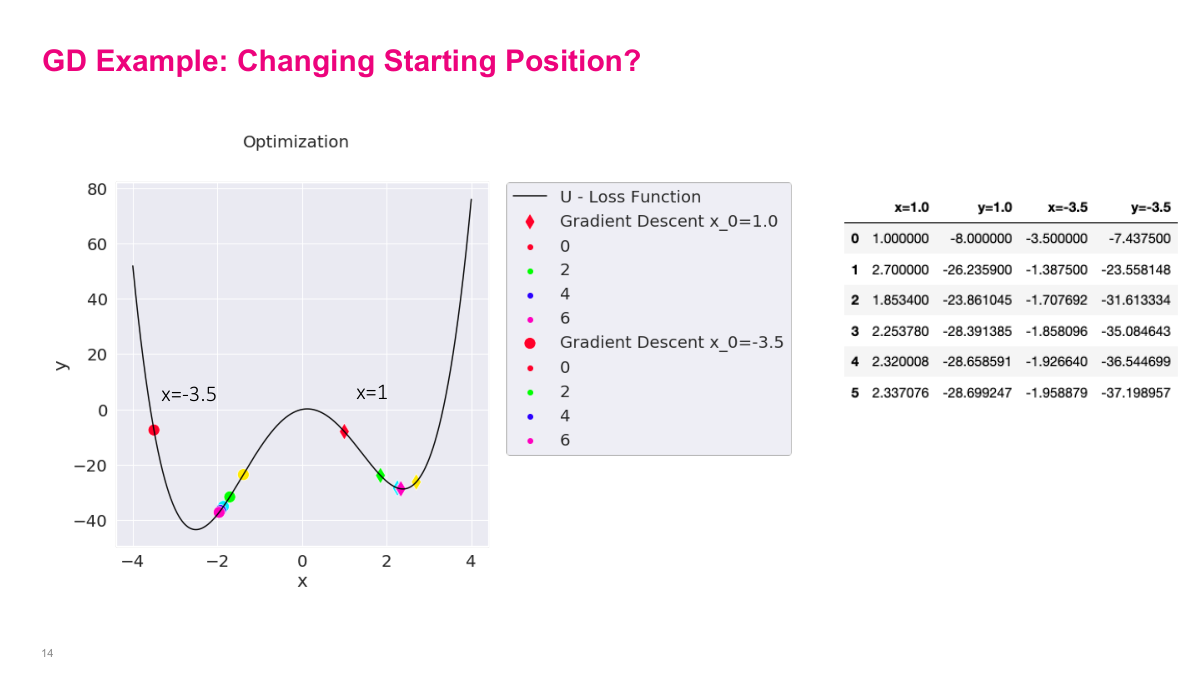
Now things get interesting when we change the starting position. Starting at negative 3.5, the algorithm takes a big initial step, overshoots the nearby local minimum, but then the negative gradient pulls it back, and it eventually settles into that local minimum. Starting at 1, the behavior is different — it overshoots in the other direction, oscillates back and forth, and eventually settles into a different local minimum. This illustrates a critical point: the initial starting position matters. Since gradient descent only guarantees convergence to a local minimum, not the global minimum, where you start determines where you end up. In this example, one starting point leads to a good local minimum while the other leads to a suboptimal one — not the global minimum at all. This is a fundamental challenge in deep learning, where loss surfaces are highly non-convex with many local minima. The choice of initialization can significantly impact the final solution quality.

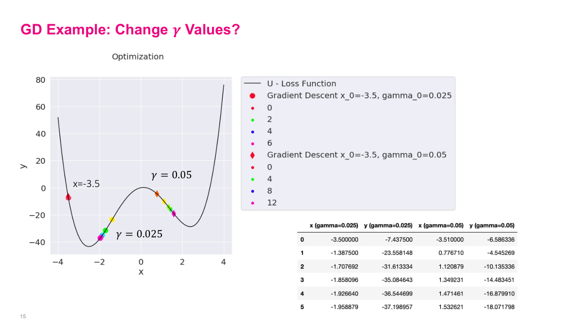
Step size makes a big difference in gradient descent. Here we compare two step sizes: gamma of 0.05 and gamma of 0.025, both starting from the same position of negative 3.5. Notice this slope is very steep, so the gradient is large. With a step size of 0.05, we take a big step and jump all the way across to a completely different part of the curve. The larger step size causes us to overshoot, potentially missing important minima along the way. This demonstrates why choosing the right step size is critical — the steepness of the function interacts with your step size to determine where you actually land after each update. A step that seems reasonable on a gentle slope can send you flying when the gradient is large.

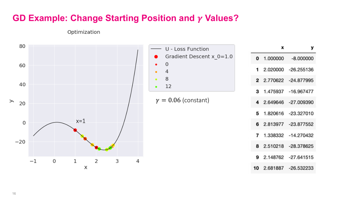
With the smaller step size of 0.025, we actually stay in the local minimum and descend properly. The larger step size of 0.05 causes us to jump right over it. This is the fundamental tradeoff: too large a step size and you overshoot minima or oscillate back and forth. Too small and convergence takes forever. This is one of the key things you have to figure out in practice. In neural networks, this step size is called the learning rate, and it's quite fiddly to get right. The last example drives this home — with a constant step size that's too large, the algorithm bounces back and forth across the minimum indefinitely, never converging. The theoretical guarantee of reaching a local minimum actually requires shrinking gamma over time. A student asked whether a large step size might accidentally find the global minimum by skipping local ones — yes, that's possible, but it's really just luck depending on your starting position and step size.

Let's review the key concepts from this section on gradient descent. First, what is an objective or loss function? It's the thing we're trying to minimize or optimize. In a machine learning context, the loss function measures the difference between what our model outputs and what we expect — the gap between predictions and actual values. Second, why are optimization problems hard? Because we're dealing with non-convex functions, and we might fall into a local minimum instead of finding the global minimum. We simply don't have reliable methods to find global minima of non-convex functions. Third, explain the intuition behind gradient descent. You take steps in the direction of the negative gradient — essentially walking downhill on the loss surface. With appropriately sized steps and some mild assumptions, you'll converge to a local minimum. These three concepts form the foundation for everything that follows.

Now we move to stochastic gradient descent, which adds some complexity. The key questions to keep in mind: What's the difference between gradient descent and stochastic gradient descent? What is a mini-batch? What are hyperparameters, and which ones do we tune? What effect does varying the mini-batch size have?

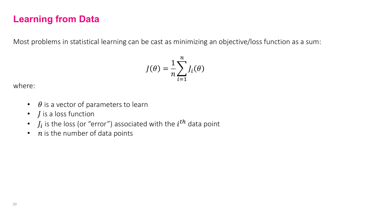
Maximizing the likelihood is equivalent to minimizing the negative log of the likelihood function. Here's the key insight: if you're maximizing a function, you're also maximizing the log of that function — they have the same optimal point. But taking the log transforms multiplications into additions. Remember, the likelihood is a product of individual probabilities, and the log of a product equals the sum of the logs. Additions are much easier to work with computationally and mathematically than multiplications. So we take the log likelihood, which converts our product of probabilities into a sum of log probabilities. Since maximizing the log likelihood is the same as minimizing the negative log likelihood, we end up with a minimization problem that's a sum over individual terms — one for each data point. This is why you see loss functions written as summations: it comes directly from the negative log likelihood formulation of maximum likelihood estimation.

The negative log likelihood gives us a loss function that's a summation over individual data points: minimize the sum from i equals 1 to n of the negative log probability for each observation. This summation structure is fundamental to understanding why stochastic gradient descent works. Because our total loss is just a sum of individual losses — one per data point — we can approximate the total gradient by computing gradients on subsets of the data rather than the entire dataset. Each individual term contributes independently to the total sum, which means we can get a noisy but unbiased estimate of the full gradient by sampling. This mathematical property of the loss function being decomposable into a sum over data points is what makes stochastic methods possible and practical for large-scale machine learning.

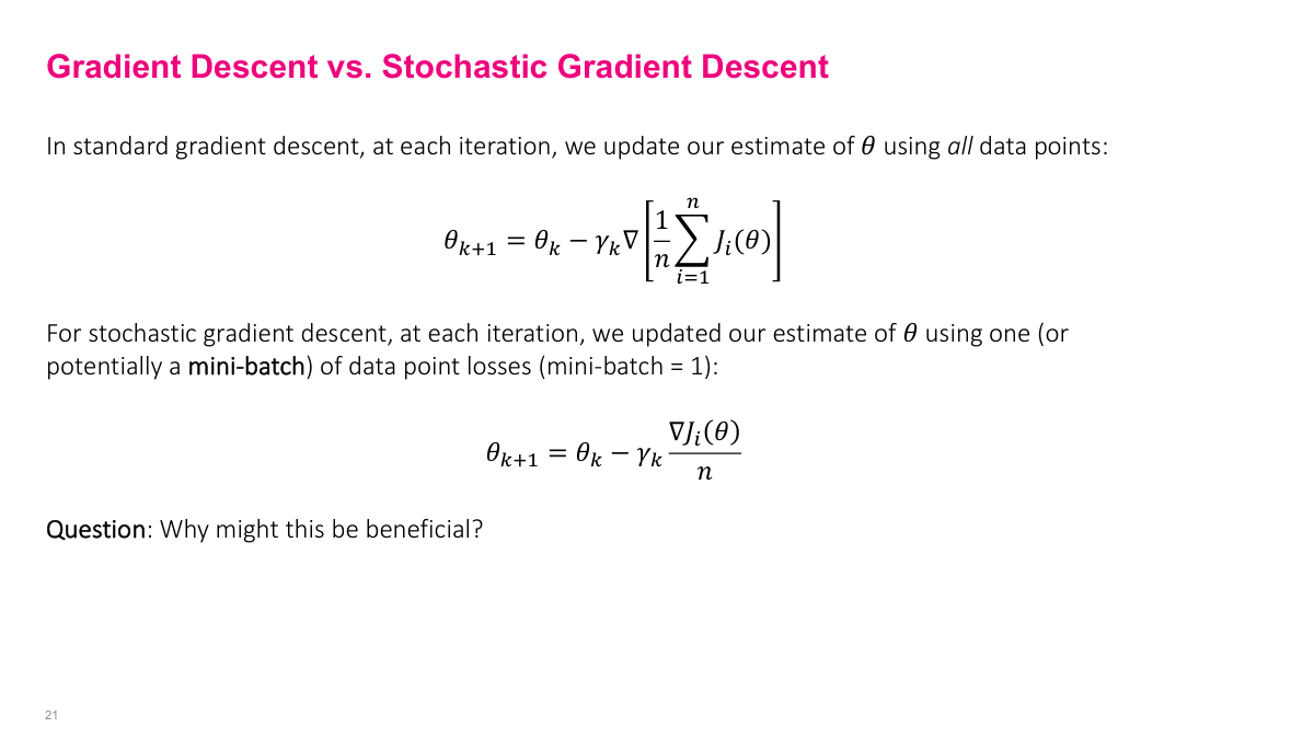
The key distinction between gradient descent and stochastic gradient descent comes down to how we compute the gradient at each step. In standard gradient descent, we compute the gradient using all n data points in our dataset — the full sum. This gives us the exact gradient, but it's computationally expensive when n is large. Stochastic gradient descent instead samples a subset of data points — a mini-batch — and computes an approximate gradient from just those examples. Because the loss function is a sum over individual terms, this sampled gradient is a noisy but unbiased estimate of the true gradient. The tradeoff is clear: we get much cheaper updates at the cost of noisier gradient estimates. In practice, this noise can actually be beneficial — it helps escape shallow local minima and explore the loss landscape more broadly. The mini-batch size becomes a key hyperparameter that controls this tradeoff between computational cost and gradient accuracy.

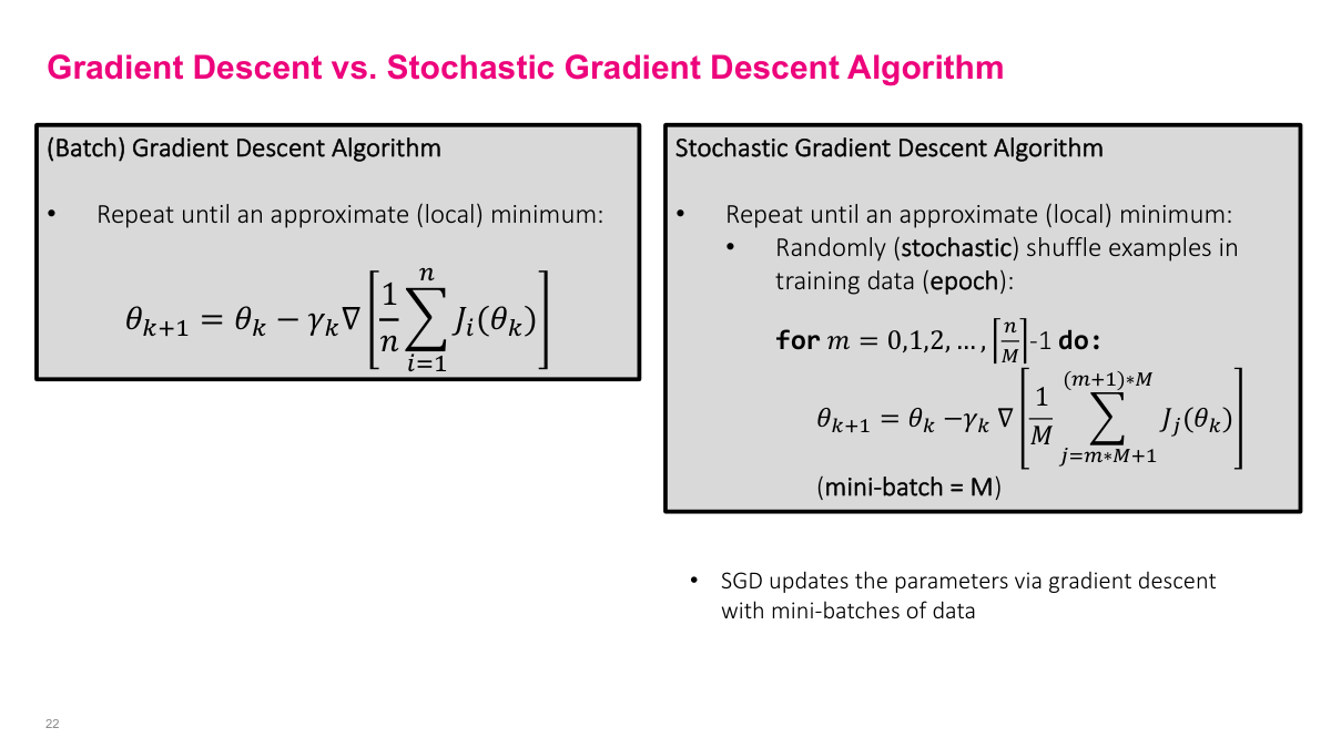
I want to compare two fundamental optimization algorithms here. On the left, we have the standard (Batch) Gradient Descent Algorithm, where we repeat until we reach an approximate local minimum. The update rule is theta_{k+1} = theta_k minus gamma_k times the gradient of the average cost over all n training examples. Notice that every single update requires computing the gradient over the entire dataset. This becomes extremely expensive when n is large. On the right, I'm showing you the Stochastic Gradient Descent Algorithm. The key difference is that we randomly shuffle examples in the training data at the start of each epoch. Then for each mini-batch of size M, we update the parameters using only that subset of data. So SGD updates the parameters via gradient descent with mini-batches of data, making each iteration much cheaper computationally while still converging to a good solution.

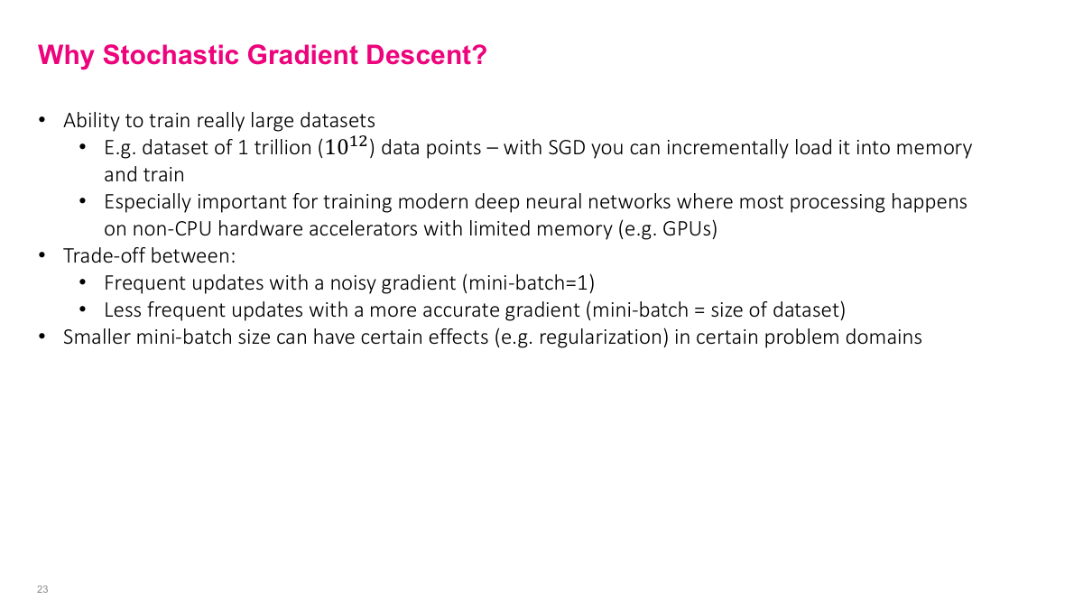
So why do we use stochastic gradient descent instead of regular gradient descent? The biggest reason is the ability to train on really large datasets. Imagine you have a trillion data points — 10 to the 12 — you simply cannot load all of that into memory at once. With SGD, you can incrementally load mini-batches into memory and train on them one at a time. This is especially important for modern deep neural networks where most of the computation happens on GPUs or other hardware accelerators that have limited memory compared to your full dataset.

There's a fundamental trade-off with mini-batch size. On one end, a mini-batch of 1 gives you very frequent updates but with a noisy gradient estimate. On the other end, setting the mini-batch equal to the full dataset size gives you less frequent updates but a more accurate gradient — that's just regular gradient descent. You're always balancing between update frequency and gradient quality. Interestingly, smaller mini-batch sizes can also have a regularization effect in certain problem domains, which can actually help generalization.

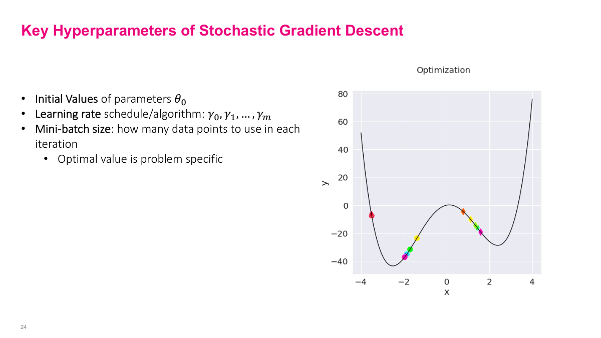
Now let me walk you through the key hyperparameters of Stochastic Gradient Descent that you need to tune carefully. First, we have the initial values of parameters -- where you start in the parameter space matters significantly, especially for non-convex problems. Second is the learning rate schedule or algorithm. Notice I'm writing this as a sequence, not a single value, because the learning rate can and often should change over the course of training. Third is the mini-batch size, which determines how many data points to use in each iteration. The optimal value is problem specific. Looking at the optimization plot on the right, you can see how gradient descent navigates a function with multiple local minima. The colored dots show the trajectory of the optimization steps. You can see it moving downhill, getting attracted to a local minimum, and then depending on the hyperparameters, it might settle in different valleys. This illustrates why initial values and learning rates are so critical to where you end up.

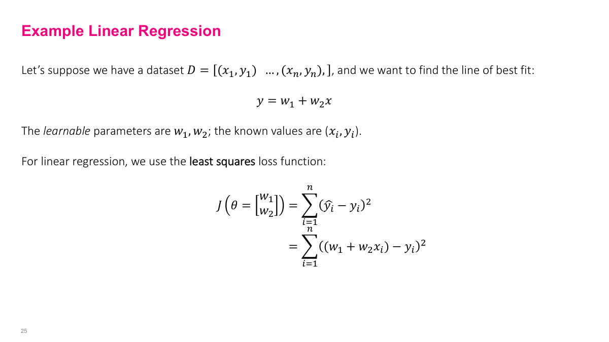
Let's walk through a concrete example with linear regression to see how all of this fits together. Suppose we have a dataset D of n pairs — each pair is an x value and a y value — and we want to find the line of best fit: y equals w1 plus w2 times x. The learnable parameters here are w1 and w2 — those are what we're trying to optimize. The x and y values are known from our data.

For linear regression, we use the least squares loss function. Our objective J is the sum from i equals 1 to n of y-hat minus y squared — that's the squared difference between our prediction and the actual value, summed over all data points. Substituting in our linear model, each y-hat is just w1 plus w2 times x_i, so the loss becomes the sum of (w1 + w2*x_i - y_i) squared. Notice that this loss is a sum over individual data points, exactly the structure we discussed earlier that makes stochastic gradient descent possible.

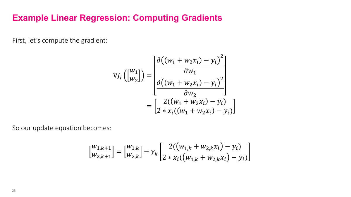
Now let's compute the gradient for our linear regression example. The gradient of the loss for a single data point i is a vector of partial derivatives — one with respect to w1 and one with respect to w2. When we take the derivative of (w1 + w2x_i - y_i) squared with respect to w1, we get 2 times (w1 + w2x_i - y_i) by the chain rule. For the partial with respect to w2, we get an extra x_i factor out front: 2x_i times (w1 + w2x_i - y_i). That gives us our gradient vector.

With the gradient in hand, our update equation becomes straightforward. At each step k, we update our parameter vector — w1 and w2 — by subtracting the learning rate gamma_k multiplied by the gradient. So w1 at step k+1 equals w1 at step k minus gamma_k times 2 times the prediction error, and w2 at step k+1 equals w2 at step k minus gamma_k times 2*x_i times the prediction error. This is the concrete mechanics of how gradient descent updates work for linear regression.

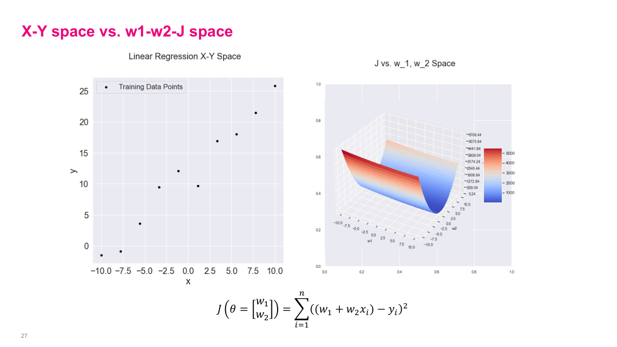
I want to show you the important distinction between X-Y space and parameter space. On the left, we have our familiar Linear Regression X-Y Space showing the training data points scattered in two dimensions. On the right, I'm showing you the same problem but viewed from the parameter space perspective. Our cost function is a squared error loss for a linear model with intercept w_1 and slope w_2. The 3D surface plot shows how the cost varies as we change w_1 and w_2. Notice it forms a bowl shape -- this is characteristic of convex optimization problems in linear regression. The color gradient from blue to red indicates low to high cost values. The contour plot below shows the same surface from above. When we perform gradient descent, we're essentially rolling down this surface trying to find the minimum point in this parameter space, which corresponds to the best-fit line in the X-Y space.

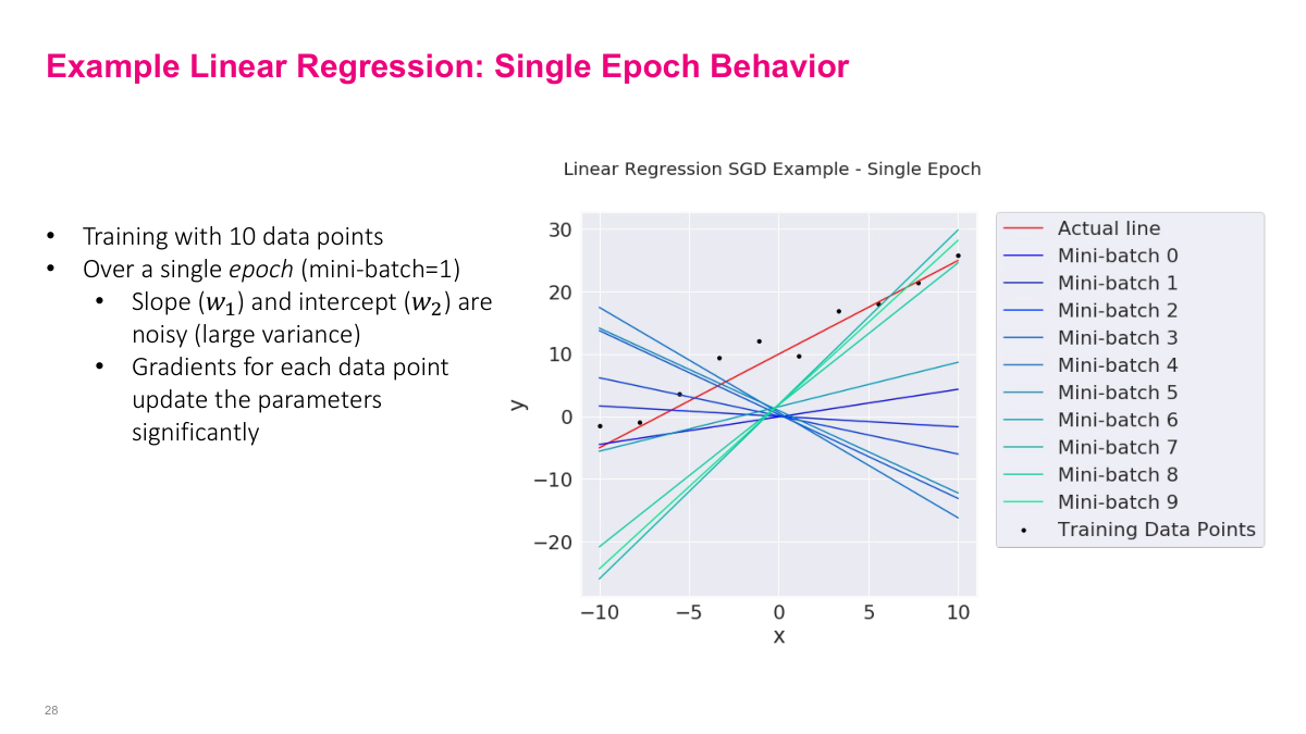
Here I'm demonstrating what actually happens during a single epoch of SGD on our linear regression example. We're training with just 10 data points and using a mini-batch size of 1, meaning each individual data point triggers a parameter update. Look at the plot -- the red line is the actual underlying relationship, and each colored line represents the fitted model after processing each successive mini-batch. You can see that the slope and intercept are incredibly noisy with large variance. The lines swing wildly from one mini-batch to the next. This is because gradients for each data point update the parameters significantly -- a single data point can push the model in a very different direction than the previous one. This is the fundamental trade-off with SGD: each update is computationally cheap, but individually noisy. Over many epochs, however, these noisy updates average out and the model converges. The stochasticity can actually help escape shallow local minima.

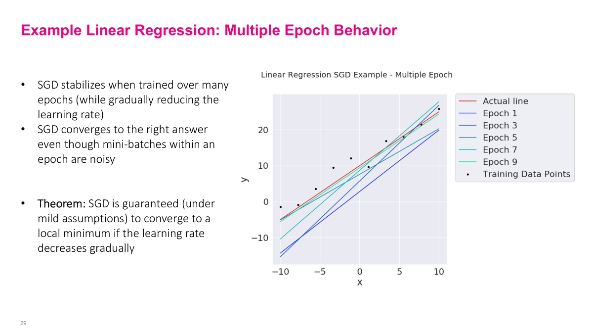
I want to show you what happens when we run SGD over multiple epochs instead of just one. Remember on the previous slide, a single epoch with mini-batch size of 1 produced wildly different regression lines — the parameters were bouncing around with huge variance. But look at what happens as we train over many epochs while gradually reducing the learning rate. The fitted lines for epochs 1, 3, 5, 7, and 9 progressively converge toward the actual line shown in red. By epoch 9, we're essentially right on top of the true relationship. This is the key insight: even though individual mini-batch updates within an epoch are noisy, SGD converges to the right answer over multiple passes through the data. There's actually a theorem that guarantees this — under mild assumptions, SGD will converge to a local minimum as long as the learning rate decreases gradually over time. The decreasing learning rate is critical because it lets the algorithm take big steps early on to get in the right neighborhood, then smaller and smaller steps to settle into the optimum.

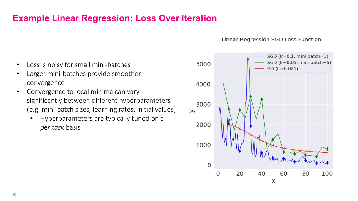
Now let me show you the loss function over training iterations for different SGD configurations compared to standard gradient descent. The green line is SGD with learning rate 0.1 and mini-batch size of 1 — notice how incredibly noisy it is, with massive spikes in the loss. It does trend downward but the individual updates are all over the place. The blue line uses a smaller learning rate of 0.05 with mini-batch size of 5, and you can see it's noticeably smoother while still converging. The red line is full-batch gradient descent with learning rate 0.025, which gives us the smoothest curve. This illustrates a fundamental tradeoff: larger mini-batches give you smoother, more stable convergence, but smaller mini-batches are computationally cheaper per step. The convergence behavior can vary significantly depending on your choice of hyperparameters — mini-batch size, learning rate, and initial values all matter. This is why hyperparameters are typically tuned on a per-task basis. There's no universal setting that works for every problem.

Let me wrap up this section with some review questions to make sure you've got the key concepts. First, what's the difference between gradient descent and stochastic gradient descent? Remember, standard GD computes the gradient over the entire dataset, while SGD uses a subset of the data — either a single sample or a mini-batch. Second, what exactly is a mini-batch? It's simply a small random subset of your training data that you use to estimate the gradient at each step. Third, what hyperparameters do we need to tune for SGD? The main ones are the learning rate, the mini-batch size, and the number of epochs. Finally, what effect does varying the mini-batch size have? As we just saw, smaller mini-batches give noisier but cheaper gradient estimates, while larger mini-batches give smoother updates but cost more computation. At the extreme of using the full dataset, you recover standard gradient descent. These are the fundamental concepts you need to understand before we move on to training neural networks.