Lecture 03: Architecture

This section covers the mechanics of training neural networks using stochastic gradient descent. We'll walk through how to define loss functions, how to compute gradients using computational graphs, and what forward and backward passes actually do. These are foundational concepts you should be able to explain off the top of your head if you work with neural networks.

The key questions for this section: What are some typical loss functions for real-valued outputs versus categorical outputs? What is a computational graph? How does a computational graph help us compute gradients? And what is a forward and backward pass in the context of neural networks? These should all be straightforward to answer if you understand the material.

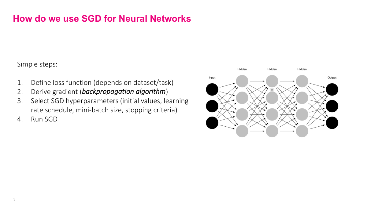
The process is the same as regular stochastic gradient descent. We define a loss function -- though now it may aggregate across multiple output nodes. We derive the gradient, which is the hard part for complex neural networks. Then we select SGD hyperparameters -- initial weights, learning rate, schedule, mini-batch size, stopping criteria -- and run the algorithm. Conceptually straightforward, but the interesting challenge is step two: how to actually compute the gradient of such a complicated function.

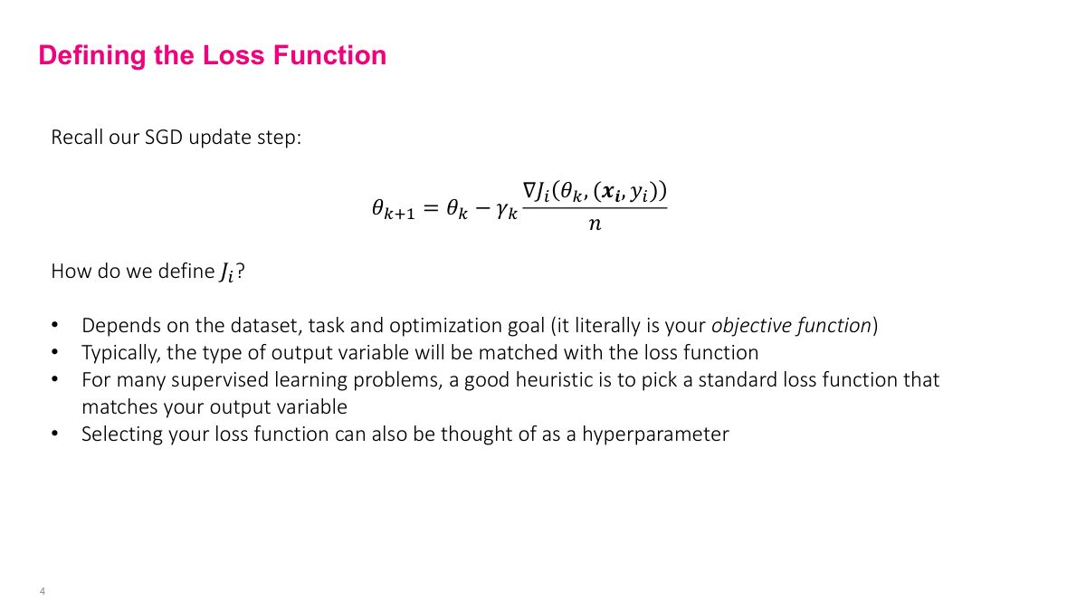
The loss function tells the algorithm what "good" means -- it defines what we're optimizing. Choosing the right one is critical because it directly determines how the model learns. The choice typically depends on your output variable. For most problems, picking one of the standard loss functions will work well. Research settings may call for more exotic choices, and you can think of the loss function selection itself as a hyperparameter.

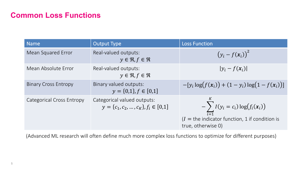
For real-valued outputs, use squared loss (MSE) or absolute error (MAE). MSE penalizes outliers more heavily. For binary outputs, use binary cross-entropy -- essentially the same as logistic regression. For categorical outputs, use categorical cross-entropy -- the generalized variant used in multinomial regression. These standard choices are reasonable starting points for most problems. One nice thing about neural networks is you can write custom loss functions if your problem demands it, giving you a lot of flexibility to customize and improve accuracy.

SGD requires computing the gradient of the loss function. As long as the function is differentiable, we can compute the gradient -- even for a thousand-layer network. The question is how. The backpropagation algorithm derives gradients backwards using the chain rule. In the early days (pre-2010), we explicitly coded the gradients for each layer by hand -- a very time-intensive process. Modern frameworks like Keras do this automatically using computational graphs and automatic differentiation, which is the more general idea I'll explain here.

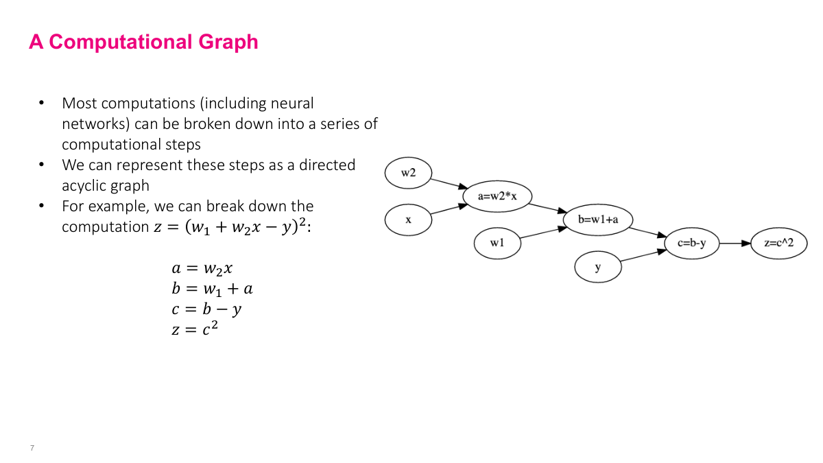
Any mathematical expression can be broken down into simpler operations and represented as a computational graph. Take a mean squared error loss: z = (w1 + w2*x - y)^2. We decompose it step by step -- multiply w2 and x to get A, add w1 to get B, subtract y to get C, square to get Z. Each node depends on its predecessors, so we execute in topological order. The key insight is that we only need derivatives of elementary operations -- addition, multiplication, squaring -- not of the full complex expression. This is how we get a computer to handle gradients programmatically instead of computing them by hand.

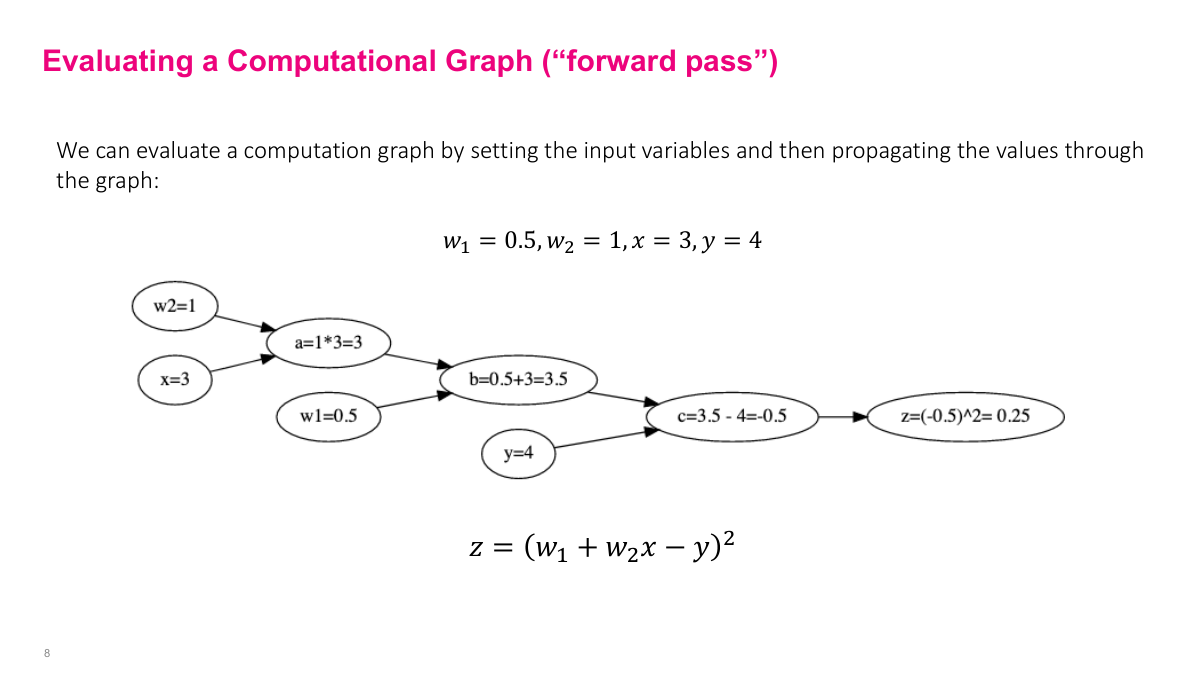
The forward pass computes all intermediate values by moving through the graph from inputs to output. Given inputs (X, Y from the dataset) and current parameter values (w1, w2 at iteration k), we populate the leaf nodes and compute each intermediate variable in order: A, B, C, then Z. This is just arithmetic. The example is simple, but the same approach works for arbitrarily complex expressions with millions of nodes -- we just move through the graph and compute everything forward. These intermediate values are stored because we'll need them for the backward pass.

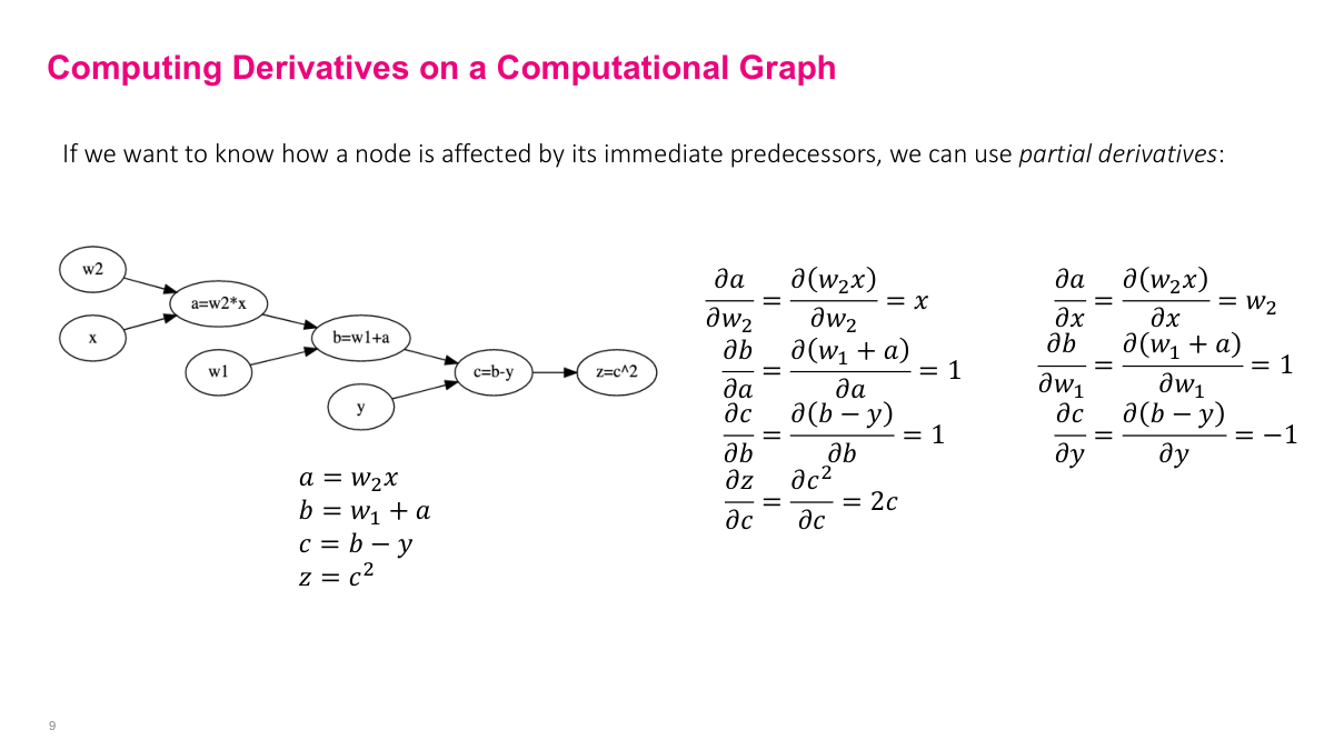
The next step is computing partial derivatives between each pair of adjacent nodes -- every edge in the graph. For example, the partial derivative of A with respect to w2 is x, and the partial of Z with respect to C is 2c. Because we already computed all intermediate values in the forward pass, we can plug them directly into these derivative expressions. The elegant part is that we only need derivatives of elementary operations (squaring, addition, multiplication, subtraction), not of the full composite function. This is a fixed, small set of derivative rules that we compute once for the graph structure.

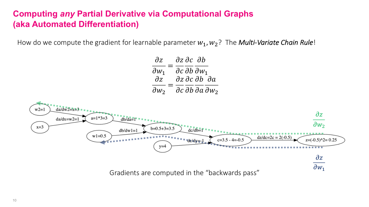
To find the partial derivative of the output Z with respect to any parameter (say w2), follow the path backward from Z to w2 and multiply the partial derivatives along each edge. This is exactly the multivariate chain rule: dZ/dw2 = (dZ/dC)(dC/dB)(dB/dA)(dA/dw2). The beauty is that the complexity of the computation is encoded in the graph -- I don't need to understand the full expression. I just need basic graph algorithms: construct the graph, do a forward pass (topological sort), then do a backward pass (path traversal), stepping back one node at a time and accumulating the gradient using the pre-computed intermediate values.

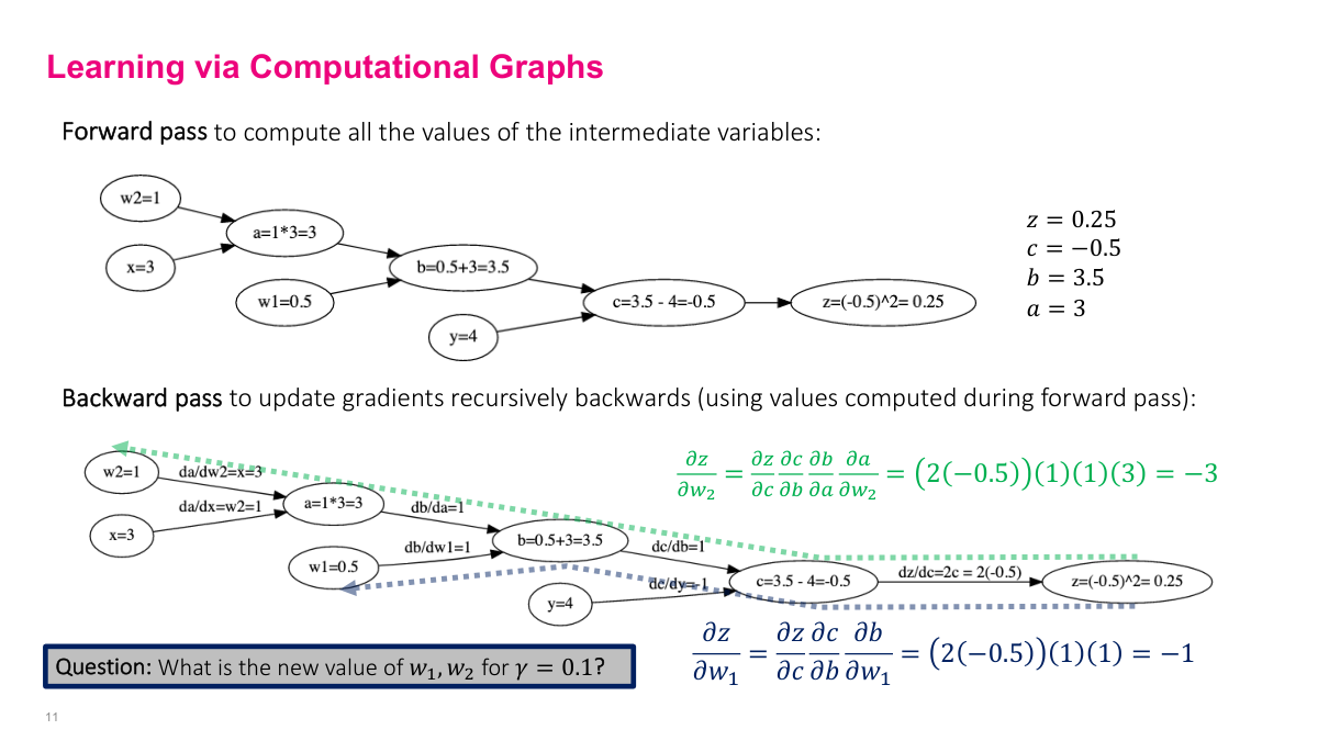
Let me walk through a concrete example to tie this back to SGD. Our parameters are w1 and w2, and we're updating them each iteration: [w1, w2]_{k+1} = [w1, w2]_k - learning_rate gradient(J). The function J is the loss -- in this case, (w1 + w2x - y)^2 for a single data point. We need to compute the gradient of this expression with respect to w1 and w2. Using the computational graph, we traverse from Z backward to each parameter, multiplying partial derivatives along each edge. The values in green and blue are the intermediate results we plug in from the forward pass. For dZ/dw1, we follow the path Z to C to B to w1. For dZ/dw2, the path goes Z to C to B to A to w2. Each backward traversal gives us the gradient value we need for the SGD update equation.

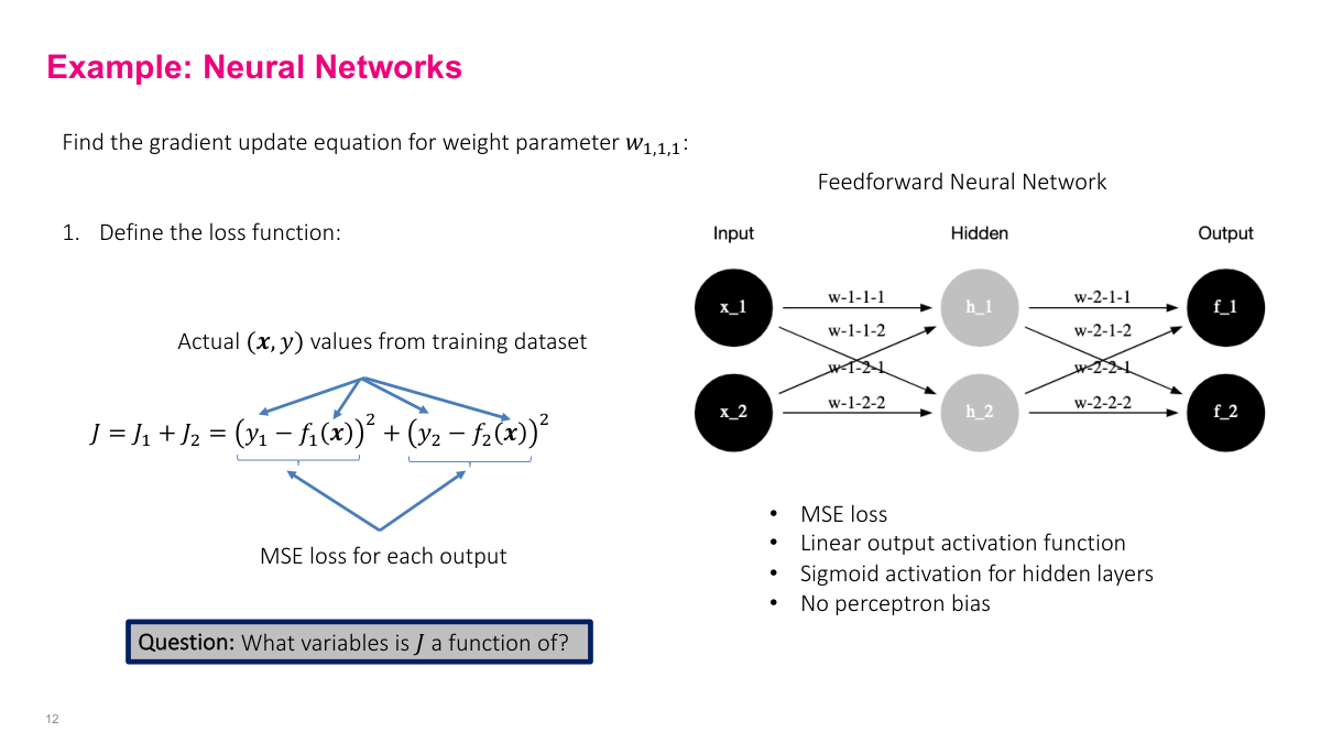
Now a slightly more realistic example: a simple feed-forward neural network with two outputs, sigmoid activation on hidden layers, linear output activation, and no biases (to keep expressions manageable). The network has eight weight parameters. The loss function is the sum of MSE from both output nodes: J = (y1 - f1)^2 + (y2 - f2)^2. An important point: J is a function of the weights, not of x and y. The x's and y's are given data points. We're optimizing the parameters to find a function that maps inputs to outputs well. This distinction trips people up because x and y are usually thought of as variables, but here they're fixed observations.

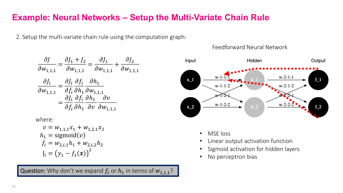
The computational graph mirrors the feed-forward network structure. To find the partial derivative of J with respect to a weight like w1,1,1, we trace the path backward: J goes to f (the output neuron), f goes to h (the hidden layer), and h connects back to w1,1,1. Since neurons combine additions and activation functions, I break them into simpler operations. The hidden layer output h1 is sigmoid(w1,1,1 x1 + w1,2,1 x2), and f is a weighted sum of hidden outputs. By writing out these equations explicitly, we can identify each edge in the computational graph and set up the chain rule for computing the full gradient.

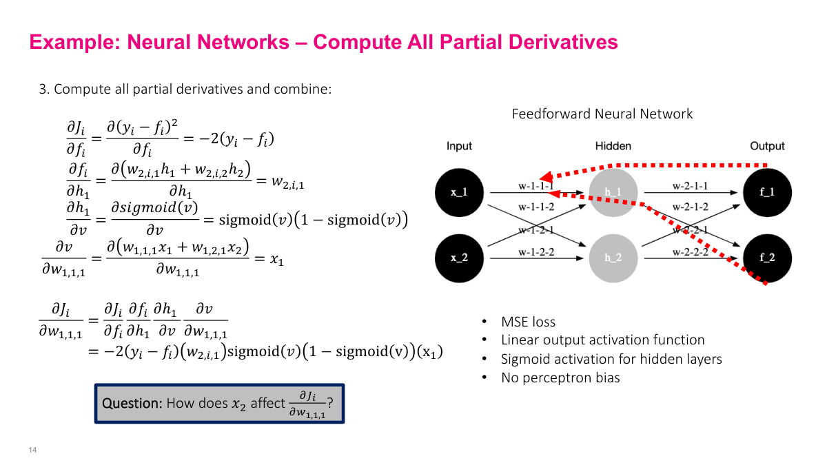
Here are the partial derivatives for each edge in the computational graph. One thing worth noting: the derivative of the sigmoid function is remarkably simple -- it's just sigmoid(x) * (1 - sigmoid(x)). Since we already have the sigmoid value from the forward pass, we don't need to recompute anything. This made sigmoid popular in early neural networks because it was computationally efficient. The full gradient expression is a product of these partial derivatives along the backward path -- exactly what we derived on the board. Every SGD iteration, we do a forward pass to get intermediate values, then plug them into these expressions to compute the gradient update.

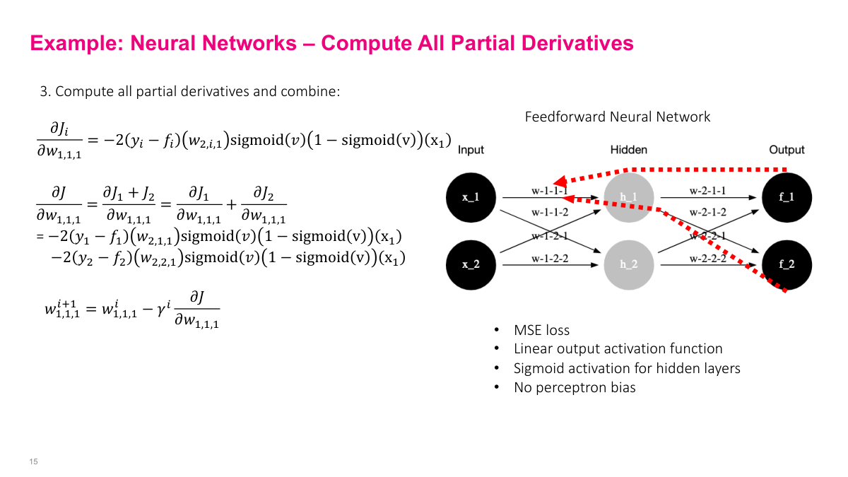
Since this network has two outputs, we need gradients from both output paths. The gradient of w1,1,1 gets contributions from both J via f1 and J via f2. Both paths contribute to the parameter update, so we combine them to get the overall gradient for that weight.

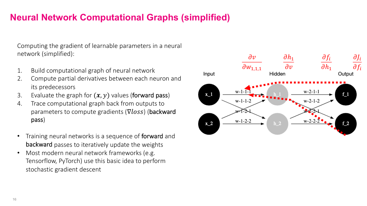
To summarize the process: build a computational graph (visually or as equations), pre-compute all partial derivatives between adjacent nodes, then iterate -- forward pass to get intermediate values, backward pass to compute gradients by plugging those values into the pre-computed derivative expressions. After the initial setup, training is just forward, backward, forward, backward -- each pair being one iteration of stochastic gradient descent.

Reviewing the key questions: Common loss functions are MSE/MAE for real outputs, binary cross-entropy for binary, and categorical cross-entropy for categorical. A computational graph breaks complex expressions into elementary operations represented as a directed graph. It helps compute gradients by enabling automatic differentiation -- computing partial derivatives on each edge and multiplying them along paths via the chain rule. The forward pass calculates all intermediate values; the backward pass uses those values to compute gradients along the edges of the graph.

Now we move from the foundational math to the practical decisions you'll actually make when building a neural network. You'll probably never compute gradients by hand, but understanding the mechanics helps when debugging. This section covers the architectural choices -- output layers, hidden layers, activation functions, weight initialization, loss functions, metrics, learning algorithms, batch size, and more.

The key questions for this section: Why do we need data preprocessing? What are some examples of output unit architectures? How many hidden layers should you have? What activation function should you use for hidden layers? Why do you generally want random weight initialization? What are some common loss functions? Why use metrics instead of loss functions for evaluation? What are some common learning algorithms? And what are some guidelines for batch size and epochs? Many of these boil down to practical guidelines for defining your neural network architecture.

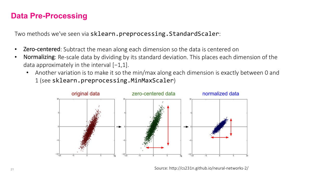
Before feeding data into a neural network, you'll want to pre-process it. Common steps include centering around zero to remove bias toward positive or negative values, and normalizing so the variance falls between -1 and 1. Scikit-learn has utilities for this. The next slide covers why this matters specifically for neural networks.

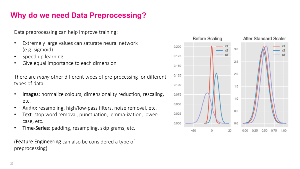
There are specific reasons preprocessing matters for neural networks. First, extremely large values can saturate activation functions like sigmoid. When sigmoid outputs are near 0 or 1, the derivative becomes approximately zero (since sigmoid'(x) = sigmoid(x) * (1 - sigmoid(x))). This kills the gradient, and learning slows dramatically. Second, preprocessing gives equal importance to each input dimension. If one feature is a million times larger than another, the model may give disproportionate importance to it in early iterations. Theoretically, a neural network can learn without preprocessing, but practically, it speeds up learning significantly and avoids pathological training behavior.

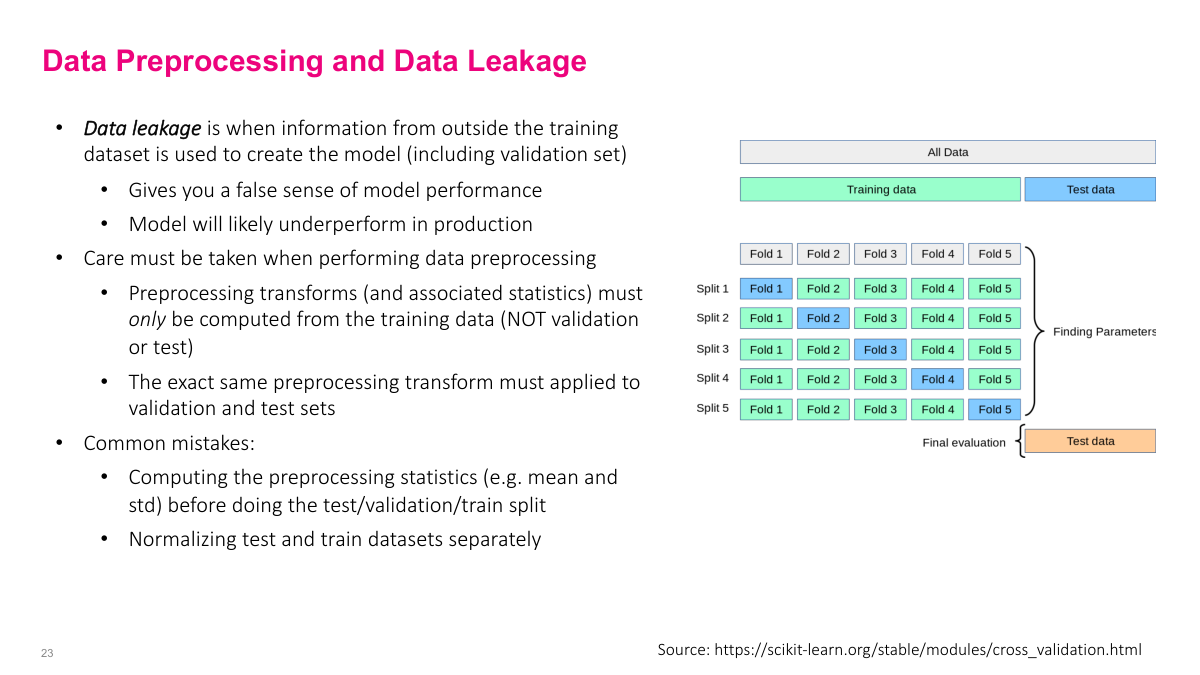
When computing preprocessing statistics like mean and variance, you must only use training data -- never validation or test data. A common mistake is computing the mean over the entire dataset before splitting, which is a form of data leakage. You're seeing values you shouldn't have access to. Data leakage is insidious in general. When someone shows me metrics like an AUC of 95%, my first assumption is data leakage -- it's the most likely explanation. In real-world problems, numbers that high are extremely rare. Many seemingly great results can be traced back to preprocessing mistakes. Spend serious time getting your data pipeline right -- it's probably more important than many of the modeling decisions we'll discuss.

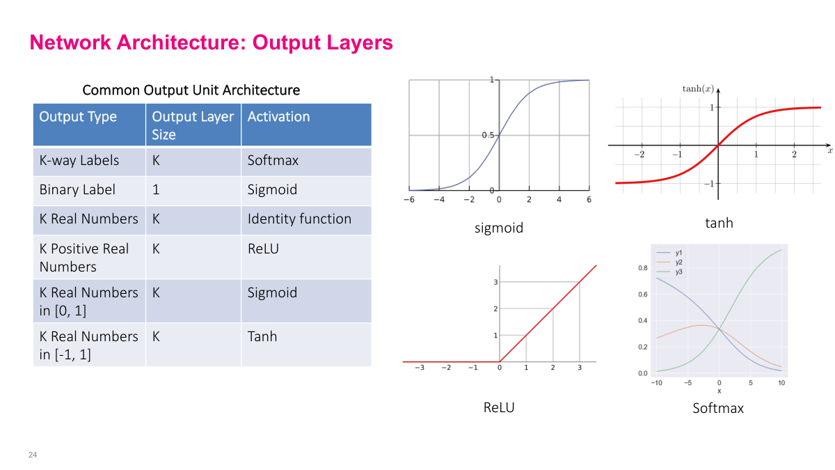
The output activation function depends on what you're modeling. Softmax for categorical outputs, sigmoid for binary labels, and various options for real numbers depending on the range. These are all reasonable defaults with well-behaved gradients. You can use more exotic choices, but these cover the vast majority of practical problems. This is one of several architectural decisions you'll need to make when building a neural network.

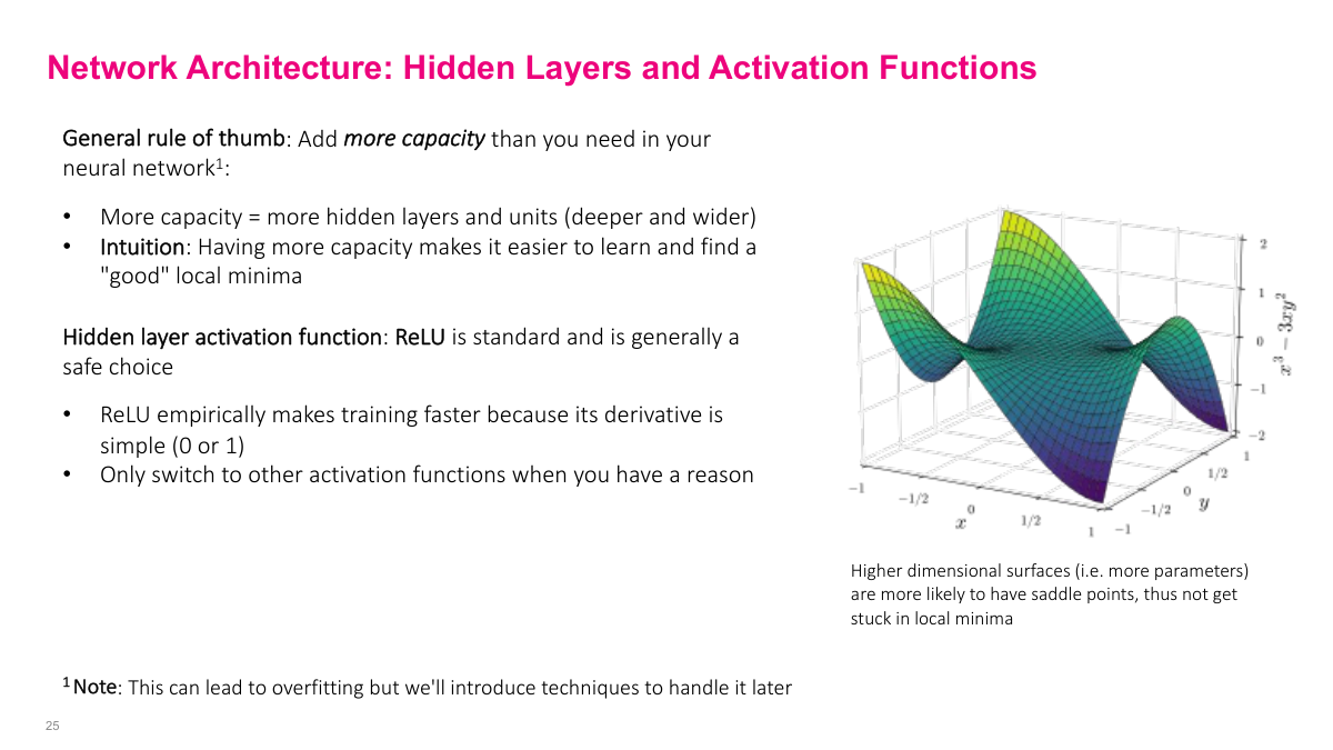
In modern deep learning, the rule of thumb is to use more hidden layers and parameters than you think you need. This is different from classical statistics where you start small and grow. The intuition: more parameters give SGD more degrees of freedom to find a good solution. With too few parameters, the learning algorithm struggles. Yes, this creates overfitting risk -- which we'll address in the next lecture -- but this over-provisioning approach is the standard methodology in deep learning. For hidden layer activation functions, start with ReLU. It's well-tested and works for 80-90% of problems without needing to think about it. Only switch away from ReLU if you have a specific reason.

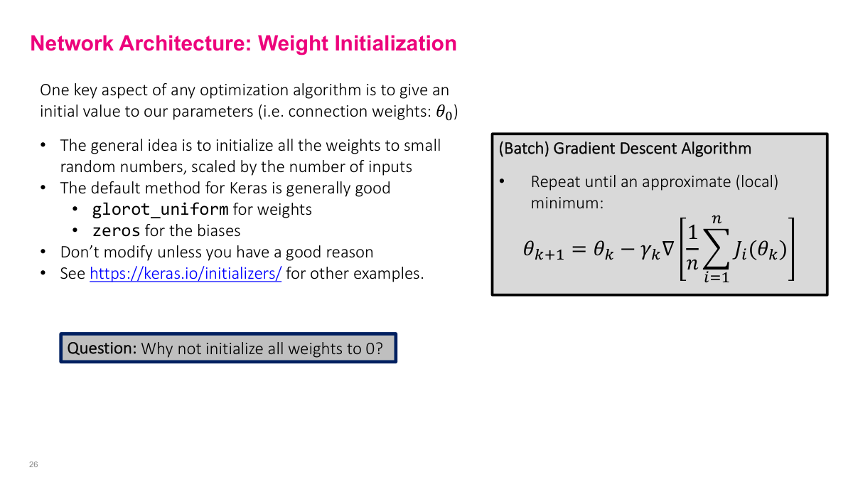
Initialize weights to small random values. Keras defaults (Glorot uniform for weights, zeros for biases) are generally good enough -- weight initialization research was a bigger deal in the early 2010s, but modern defaults work well. Why not initialize to zero? Two reasons. First, if all weights are zero, the network is symmetrical -- all outputs are the same, all gradients are the same, and the network never learns anything interesting. Second, because we multiply values together in the chain rule, having zeros or near-zeros kills the gradient entirely and stops learning. You want small but nonzero values to avoid these pathological cases.

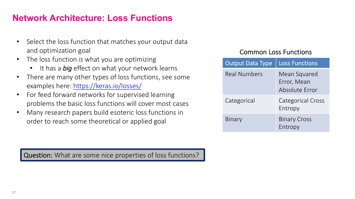
The loss function tells the network what "good" means, so it has a major effect on what the model learns. Stick with the standard choices (MSE, binary cross-entropy, categorical cross-entropy) unless you have a reason to do otherwise. What makes a good loss function? It should align with your output data type, penalize larger errors more, have well-defined gradients (otherwise you can't use it in gradient descent), be relatively smooth (no jagged discontinuities), and be easy to compute. Neural network frameworks let you define custom loss functions, which is powerful for specialized problems, but the standard options are a solid starting point.

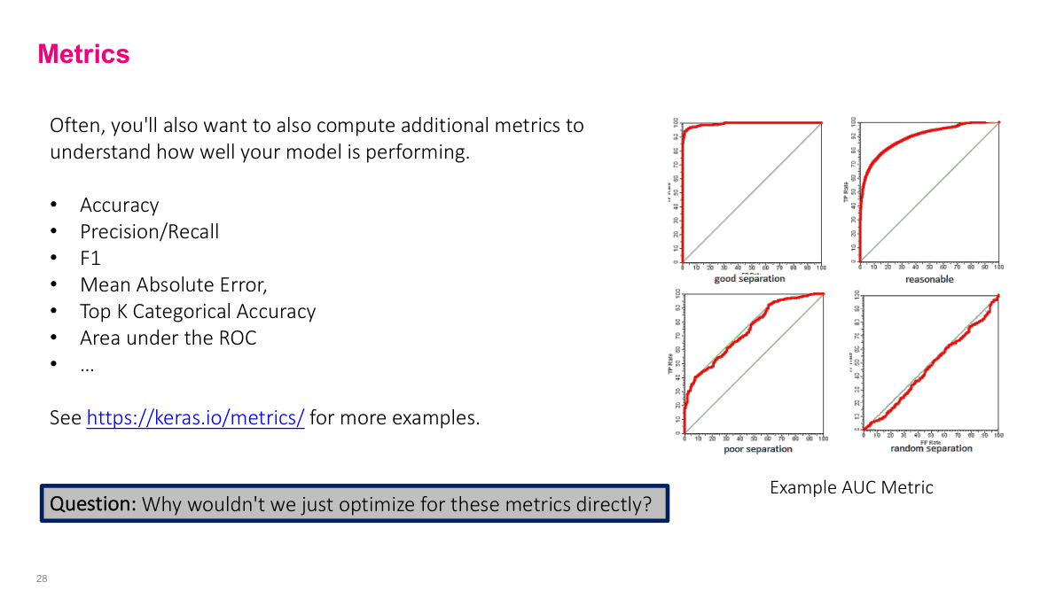
We use metrics like accuracy, precision, recall, and F1 to understand how well we're solving the problem, but we can't optimize them directly. Consider accuracy for binary classification: you either get it right or wrong, which produces a step function. How do you take the gradient of a step function? You can't -- it's not smooth. That's why we use proxy loss functions like cross-entropy that are smooth and differentiable, even though what we actually care about are metrics like accuracy or AUC. The loss function is what gradient descent can optimize; the metric is what we use to evaluate whether the model is actually solving our problem.

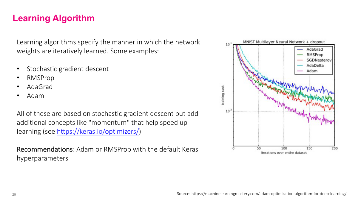
Basic SGD uses a fixed learning rate, but more advanced optimizers dynamically adjust it. Algorithms like RMSProp, AdaGrad, and Adam effectively change the learning rate by looking at previous gradient history. Adam is particularly popular -- even GPT-3 was trained with a variant of it. These optimizers learn faster than vanilla SGD because of how they adapt the learning rate. My recommendation: just pick Adam or RMSProp as a starting point. If you're pursuing deep learning seriously, understanding how these differ from basic SGD is worthwhile, but for practical purposes, the defaults work well.

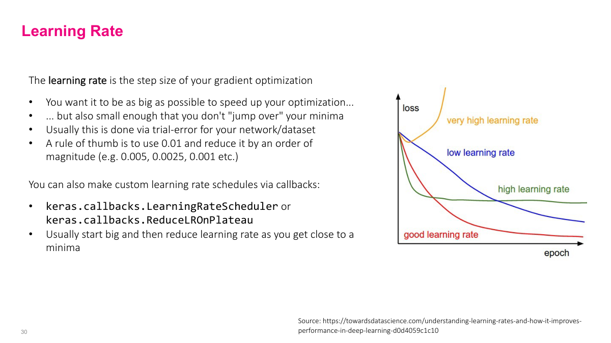
For the learning rate, start around 0.01 or 0.001. Then adjust by multiplying or dividing by 2 or 5 to find the sweet spot. You want something that learns quickly without jumping over minima. Some papers use more exotic schedules -- raising then lowering the rate -- but for straightforward problems, a simple fixed value works fine. Modern frameworks like Keras have built-in support for learning rate schedules if you need them, but a reasonable starting point and some experimentation usually gets you there.

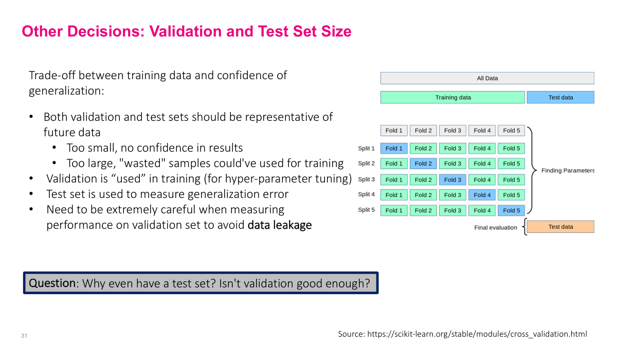
The validation set guides most of our decisions in machine learning -- how many layers, what learning rate, which hyperparameters. We use it to tune the model, and the test set to measure real performance. The critical thing to watch for is data leakage: inadvertently including information in training that gives a false sense of model quality. Common mistakes include using a column that reveals the future, or computing statistics over the full dataset before splitting. Why have a test set at all? Because we're effectively overfitting to the validation set through our hyperparameter choices. The test set is a completely independent measure that never participates in any decision during training. Without it, we don't know if our validation performance reflects true generalization.

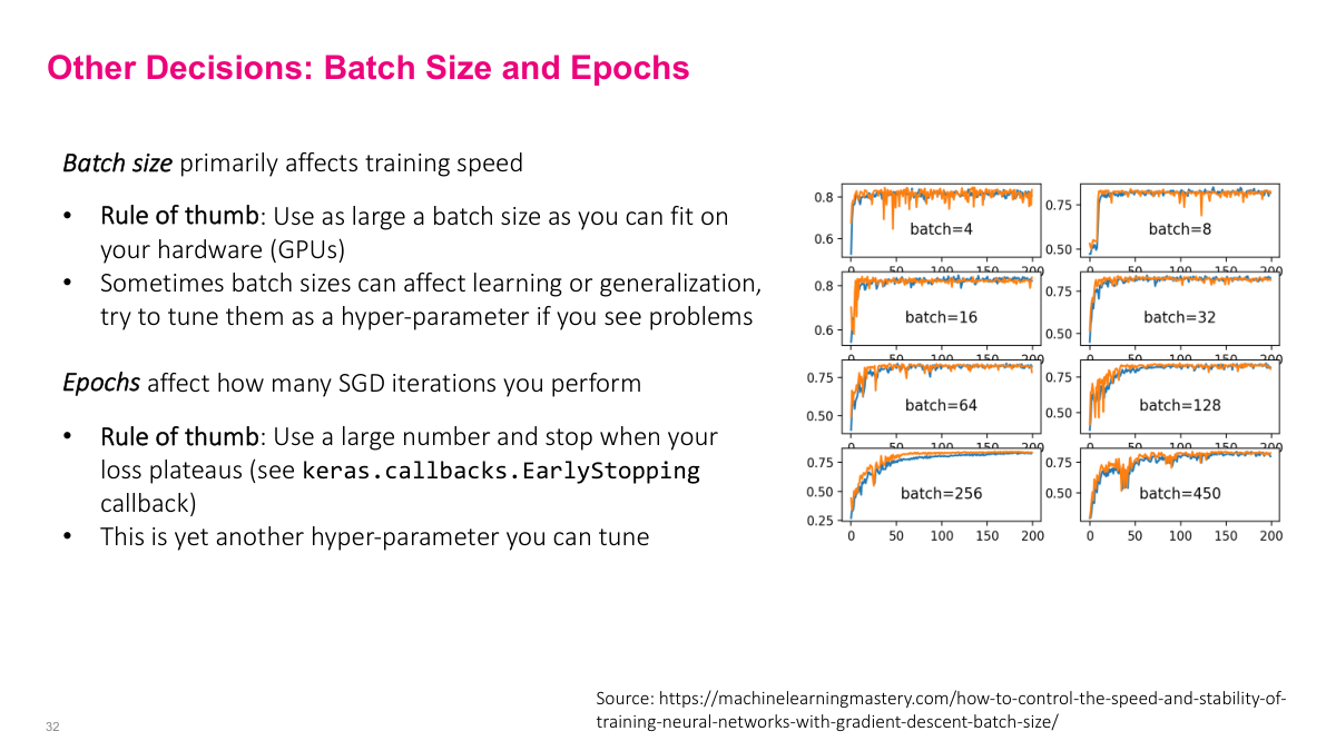
For batch size, my rule of thumb is to use the largest batch that fits in your GPU memory. Bigger batches mean faster learning and more iterations per unit time. There are fiddly optimizations, but maximizing batch size is a solid starting point. For epochs, use a large number and wait for the loss to plateau. Save model weights at checkpoints along the way -- if you overshoot and overfit at epoch 100, you can roll back to epoch 10 where the saved weights performed best. This checkpointing approach means you don't need to guess the right number of epochs in advance.

We'll cover these review questions at the beginning of the next class.