Lecture 11: Marketing II

In this section, I focus on customer data as the foundation for marketing models. The main ideas are what a customer signature is, why it is worth building one, and how to think about missing values. A lot of applied modeling problems are really data-definition problems first, so I want to ground the discussion in how we represent customers before we jump into the models that use them.

The key questions here are straightforward: what a customer signature is, why we use one, and how to handle missing values. Those three ideas capture most of the practical work in customer data. If I can define the customer properly, summarize them consistently at a point in time, and deal with incomplete data intelligently, then I have the raw material for downstream analytics and machine learning.

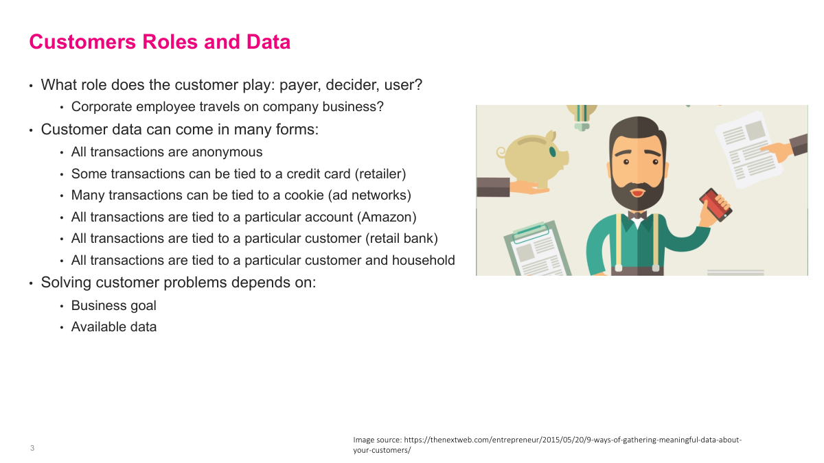
The word customer sounds simple, but it is often ambiguous. The payer, the decider, and the actual user may be different people, especially in enterprise settings. The data can also exist at very different identity levels: anonymous transactions, credit-card-linked activity, cookie-based browsing, account-level histories, or household-level relationships. That means I cannot treat customer modeling as an abstract ML problem. I need to understand the business goal and the data that are actually available, because the right definition of customer depends on both.

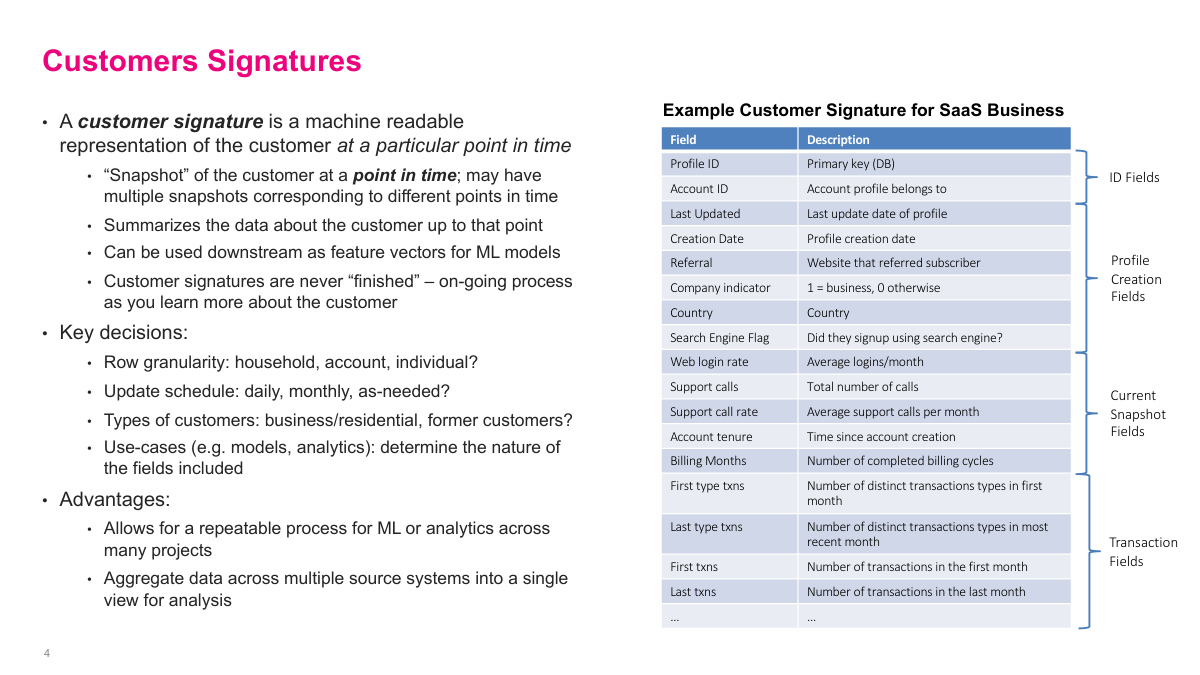
A customer signature is a machine-readable snapshot of a customer at a particular point in time. That point-in-time idea matters because customers change: their tenure, spending, products, and behavior evolve, so different snapshots can represent meaningfully different versions of the same customer. A good signature summarizes what I know up to that date and makes it reusable for analytics or ML. The design choices are practical ones: row granularity, update cadence, which customers to include, and which fields matter for the use case. The payoff is a repeatable, centralized view of the customer instead of rebuilding features from scratch for every project.

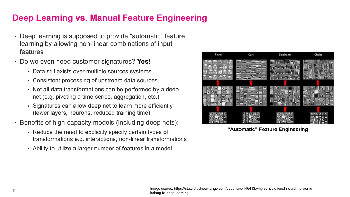
Deep learning reduces some of the need for manual feature engineering, but it does not eliminate the need for customer signatures. I still have to collect data from multiple source systems, align identities, and apply upstream transformations consistently. Some operations, like pivoting time series data or doing business-specific aggregations, are awkward or inefficient to ask a model to learn from scratch. High-capacity models are useful because they can absorb more features and learn non-linear interactions, but I still get better results when I hand them a well-constructed customer representation.

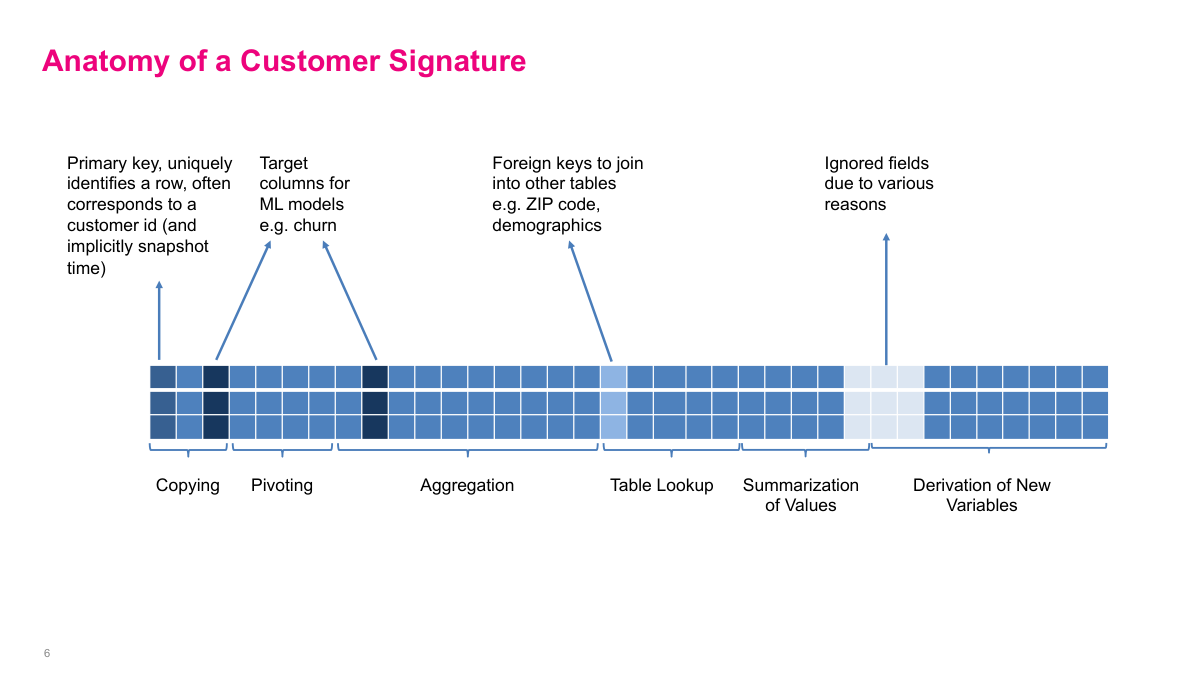
In practice, a customer signature is usually a very wide table. It includes primary keys, fields copied from source systems, pivoted time-series values, aggregated transactions, lookup fields such as demographics or ZIP-code data, summary statistics, and derived variables. Sometimes it also includes target columns for specific modeling tasks. I think of this as the source of truth for customer analytics. If this table is already tested and maintained centrally, I can build a model in a day. If it is missing, I may spend months just assembling data before the actual modeling work starts.

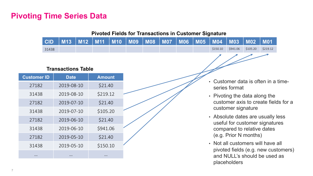
Transaction data is one of the richest customer data sources, but it is awkward because each customer has a variable number of rows. A common fix is to pivot the time series along the customer axis so that I get one row per customer and columns for relative periods such as the prior 13 months. Within each month, I aggregate amounts, often by summing them. Relative dates are usually more useful than absolute dates because they preserve recent behavior patterns like rising or falling spend. Newer customers will naturally have missing periods, so those columns need explicit null handling.

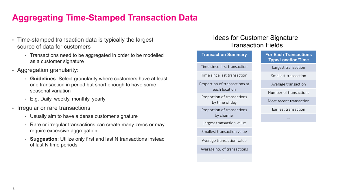
When I aggregate transaction data, I need a granularity that is dense enough to be informative but short enough to preserve seasonality. Depending on the business, that could be daily, weekly, monthly, or yearly. Beyond simple spend totals, I can derive time since first or last transaction, min and max transaction value, averages, and channel or location proportions. If transactions are rare or irregular, aggregating fixed time periods can create a signature full of zeros. In those cases, it can be better to use the first or last N transactions instead of the last N time buckets.

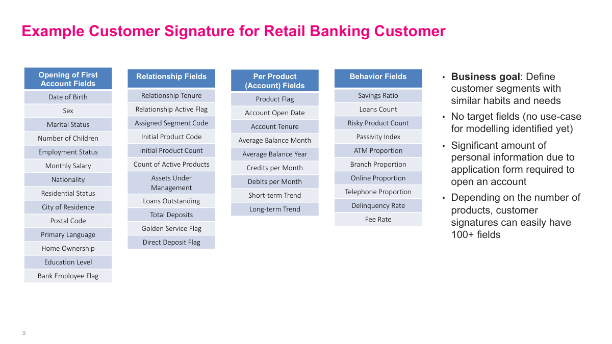
This banking example shows how wide a real customer signature can become. I may include opening-account profile fields, relationship-level fields, product-specific account variables, and behavior metrics such as savings ratio, channel usage, delinquency rate, or fee rate. Even without defining a modeling target yet, this kind of table is already valuable for segmentation and analytics. In industries with rich onboarding forms and multiple products, it is easy to end up with well over 100 fields, which is exactly why it helps to build the signature once and reuse it broadly.

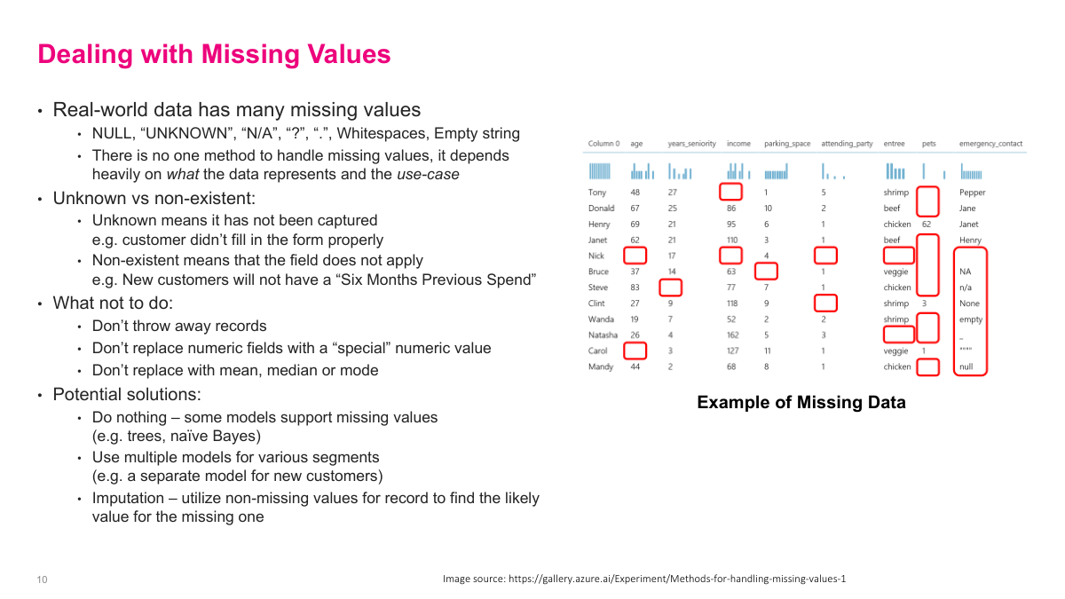
Missing values are a fact of life, and they do not all mean the same thing. Some are unknown because the data were never captured properly. Others are non-existent because the field does not apply, like a new customer with no six-month spend history. That distinction matters. As a rule, I do not want to throw away records blindly, replace numbers with a special sentinel, or default everything to the mean, median, or mode. Better options are to use models that support missingness, build separate models for segments with systematically different missing patterns, or apply more informed imputation.

The main takeaway from this section is that a customer signature is a point-in-time feature representation of the customer, and it is useful because it creates a reusable foundation for analytics and ML. Most of the hard work is upstream: defining the customer correctly, assembling data across systems, and deciding how to treat missingness. If I get that layer right, the downstream models become much easier to build and trust.

This section moves from representing customers to deciding what to do with them. I focus on the main families of targeting problems: response or propensity models, time-to-event models, and lifetime value models. The common thread is that they all try to answer the who question in marketing, but they optimize for different business outcomes and require slightly different formulations.

The questions here cover the main targeting toolkit: the three categories of targeting models, the difference between response and uplift, the role of RFM, how to formulate propensity models, and how to model revenue, time to event, and lifetime value. If I can answer those, I have a solid map of the common marketing modeling problems.

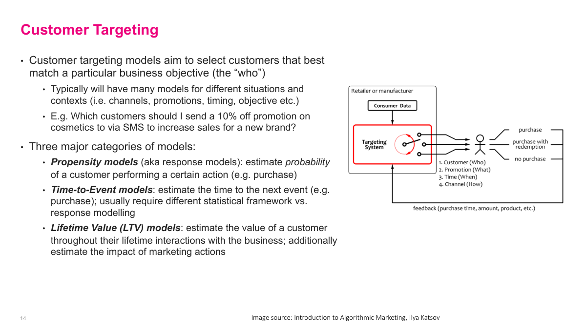
Customer targeting is about deciding who should receive a particular action under a particular context: which customer, with what promotion, through which channel, and at what time. I usually think of three model families. Propensity models estimate the probability of an action such as purchase or click. Time-to-event models estimate when that action is likely to happen. Lifetime value models estimate the long-run value of the customer. LTV is especially important because acquisition is often one of the most expensive parts of the business, so I need some estimate of long-run value to know how much I can rationally spend to win the customer.

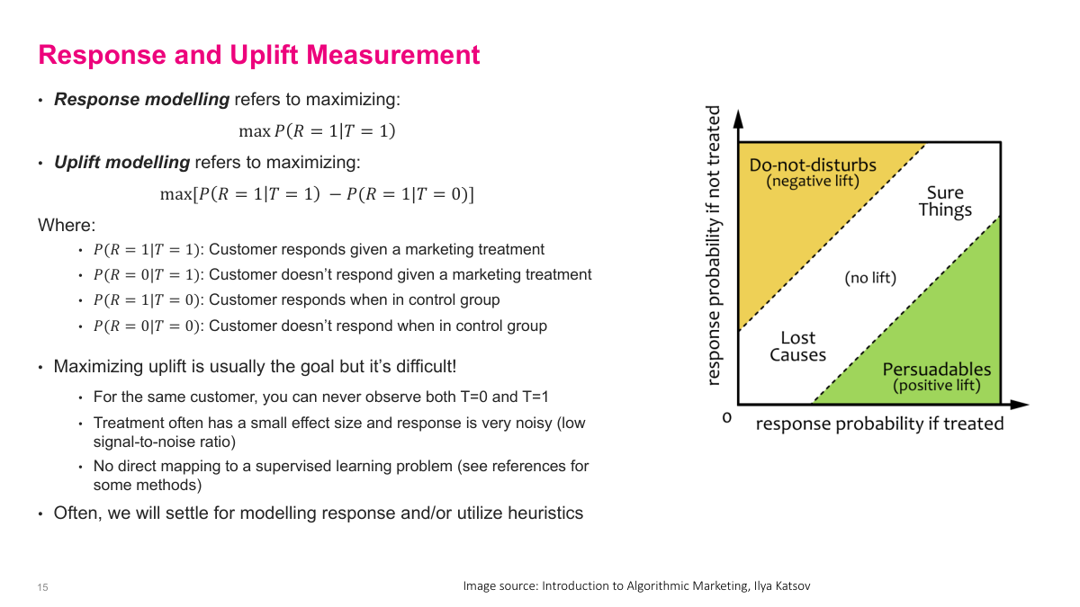
Response modeling asks for the probability of response given treatment, while uplift modeling asks for the incremental change caused by the treatment itself. That distinction is important. Some customers are sure things and will buy anyway. Others are lost causes and will not buy regardless. The most valuable group is the persuadables, where the treatment actually changes behavior. In principle I want to maximize uplift, not just raw response, but uplift is harder because I never observe both the treated and untreated outcome for the same customer, and the signal is usually noisy.

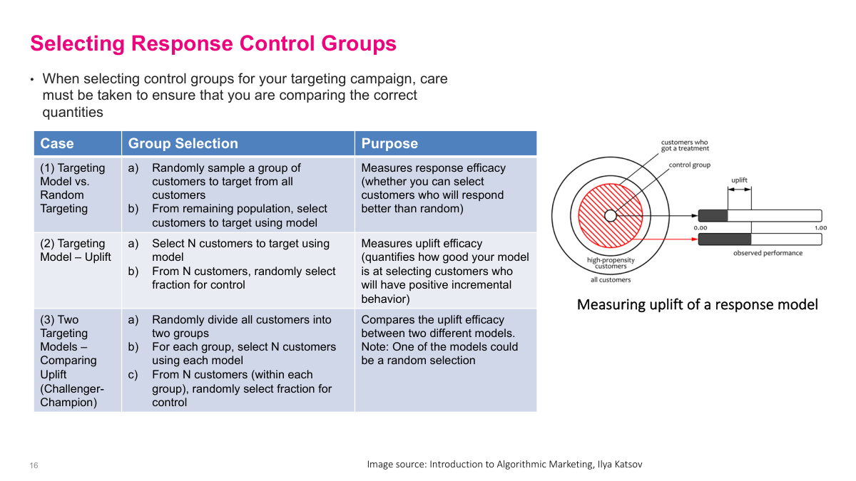
Control-group design determines what I am actually measuring. If I compare model-selected customers against a random target group, I am testing whether the model beats random targeting. If I carve out a control group from the model-selected customers, I am measuring uplift of the campaign within the targeted population. If I want a challenger-champion comparison, I need to split the population and give each model its own treatment and control structure. The key point is that a random control group is not enough by itself; I have to align the control design with the business question.

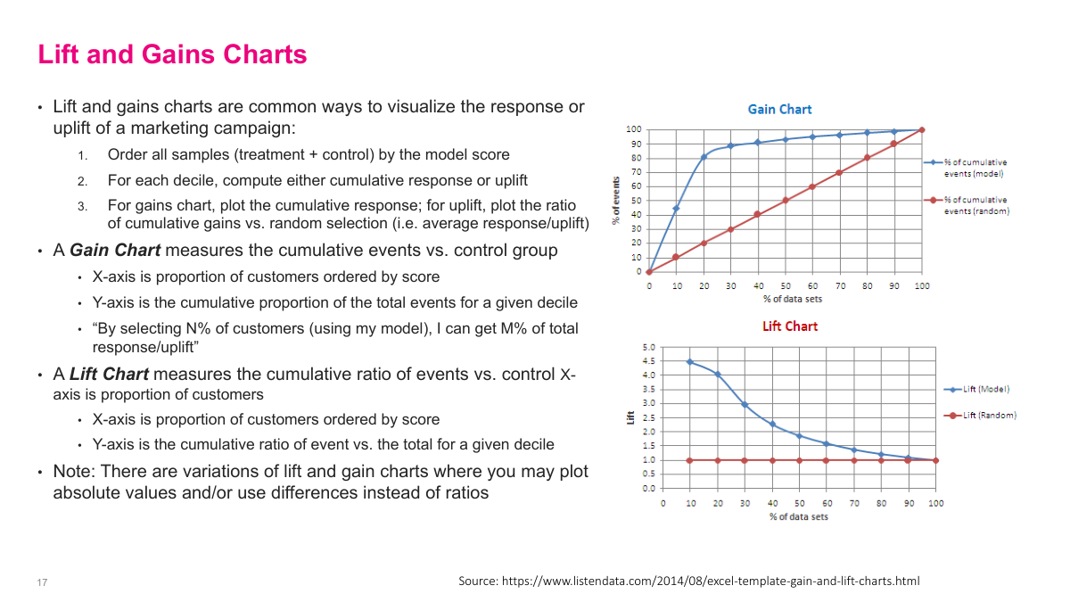
Lift and gains charts give me an intuitive way to explain targeting performance. I order customers by model score and then look at the cumulative response or uplift by decile. A gains chart tells me something like: by targeting the top 20% of customers, I capture 70% or 90% of the total response. A lift chart shows how much better that ranked selection is than random targeting. I like these views because they translate model quality directly into business terms such as how many offers I really need to send.

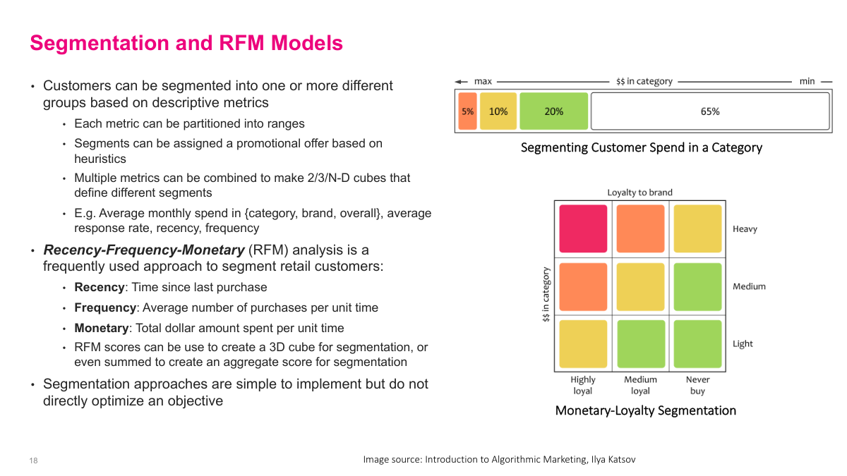
Segmentation is an older but still useful way to act on customer data. Instead of scoring each customer individually, I partition customers into groups using descriptive metrics and assign actions by heuristic. RFM is the classic example: recency, frequency, and monetary value. Those three variables are strongly associated with good customers, so they work well both as a segmentation scheme and as default model features. The downside is that segmentation is coarse and does not directly optimize an objective, but it is simple, interpretable, and often a strong baseline.

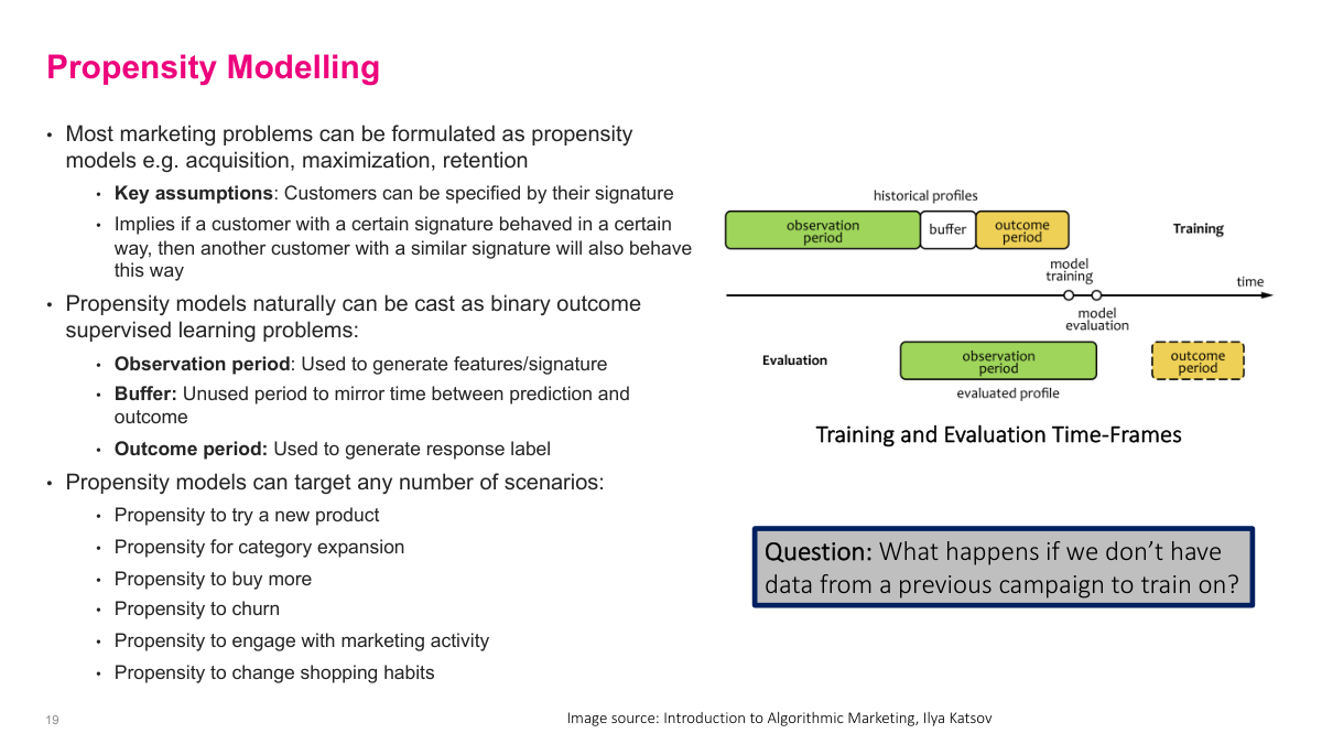
Most marketing problems can be framed as propensity models: probability of trying a product, buying more, churning, or engaging with a campaign. The important implementation detail is time. I use an observation period to build features, a buffer to reflect operational delay, and an outcome period to define the label. That is really a backtesting setup, and it avoids the leakage that happens if I randomly sample training and test points across time. The training setup should mirror production. If I do not have historical campaign data, sometimes the right answer is simply to run a smaller test campaign to collect labels.

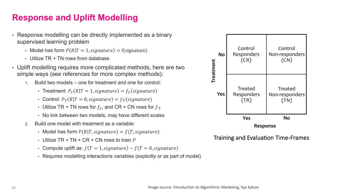
Response modeling maps cleanly to supervised learning: I take treated responders and treated non-responders and predict response from the customer signature. Uplift modeling is more awkward because it is fundamentally about the difference between treated and control outcomes. One approach is to build separate treatment and control models and subtract them, but calibration can drift across the two models. Another is to build one model with treatment as an explicit variable and compare predictions under T=1 and T=0, but that only works if the model actually learns the treatment interaction. In practice, uplift is difficult enough that I often model response and measure uplift separately.

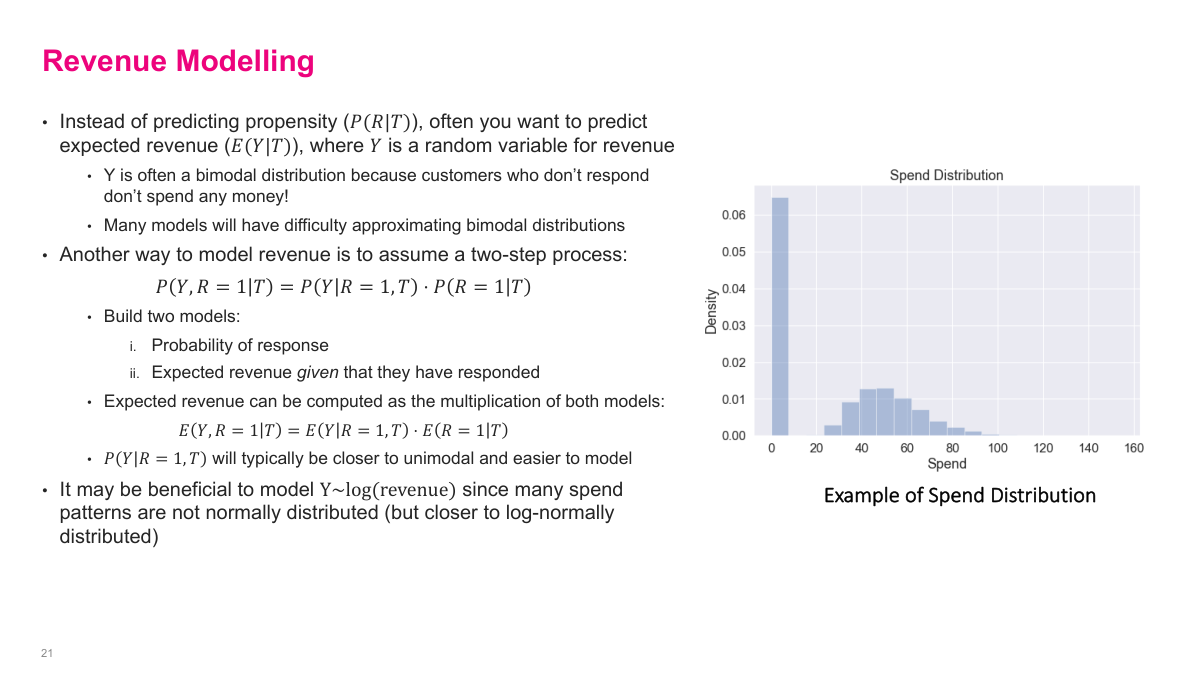
Sometimes the real objective is expected revenue, not just probability of response. The problem is that revenue is often bimodal: many customers spend nothing, while responders follow a separate right-skewed spend distribution. A useful workaround is a two-stage model. First I model the probability of response. Then, conditional on response, I model how much revenue the customer generates. Multiplying those pieces gives an estimate of expected revenue. That is usually easier than forcing one model to learn the full bimodal distribution directly, and it is often better behaved if I work on log revenue for the spend model.

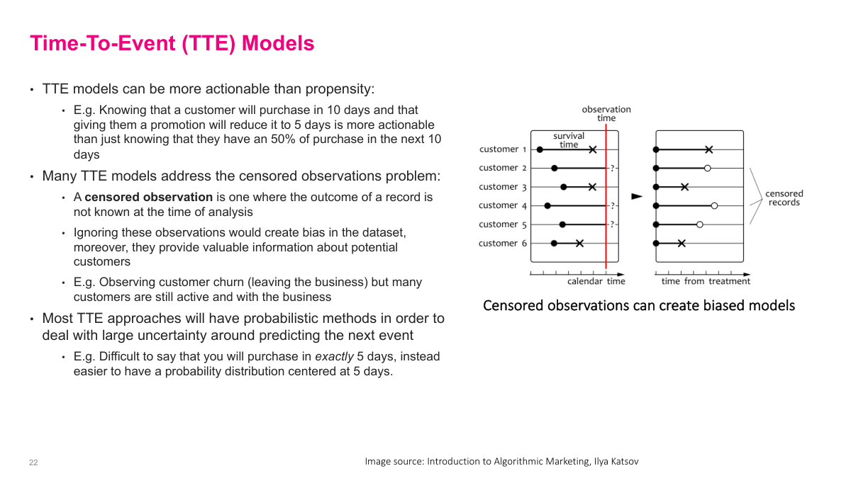
Time-to-event models ask when something will happen, not just whether it will happen. That can be more actionable than a plain propensity score. Knowing a customer is likely to purchase in 10 days, and that a treatment might shorten that delay, is often more useful operationally than knowing there is a 50% purchase chance. These models also have to deal with censored observations, where I have not yet seen the event by the time I analyze the data. Those records still contain information, so I do not want to ignore them.

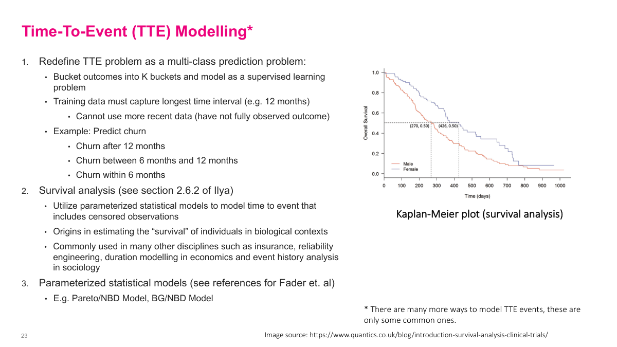
A practical way to simplify time-to-event modeling is to turn it into a supervised learning problem by bucketing the time horizon, for example churn within 6 months, between 6 and 12 months, or after 12 months. That loses some precision, but it makes the problem much easier to train and deploy. The trade-off is that I need enough history to observe the full window. If I want more statistically principled approaches, survival analysis and parameterized models such as Pareto/NBD or BG/NBD are common alternatives, especially when censored observations matter.

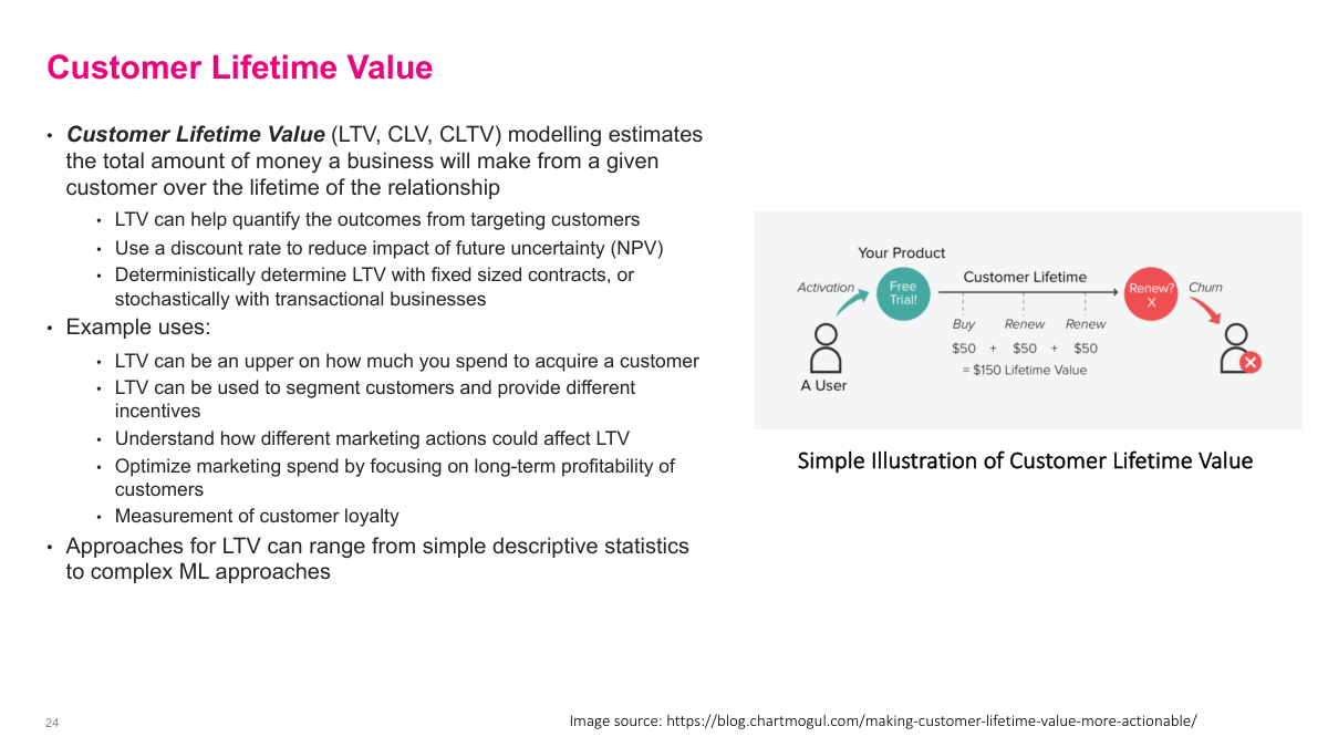
Customer lifetime value estimates how much total value a business expects to earn from a customer over the full relationship. That estimate matters because it puts an upper bound on acquisition spending, supports segmentation, and helps me reason about long-term profitability instead of short-term conversion alone. In some businesses LTV can be almost deterministic, such as fixed contracts. In more transactional settings it is stochastic, so I usually combine retention, profit, and discounting assumptions to account for uncertainty and the time value of money.

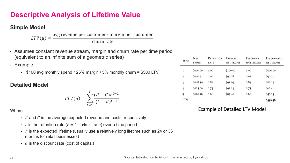
There are simple and detailed descriptive ways to estimate LTV. The simplest formula is average revenue times margin divided by churn rate, which is basically a geometric-series approximation under stable assumptions. That gives a fast back-of-the-envelope estimate for how much a customer is worth. A more detailed version uses discounted cash flow: expected revenue minus cost, multiplied by retention over time and discounted back to present value. The simple model is coarse but useful. The detailed model is richer, but only as good as the retention, cost, revenue, and discount-rate assumptions I plug into it.

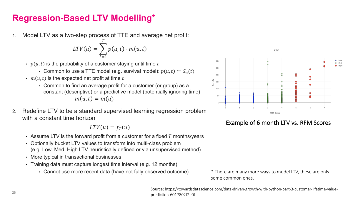
One way to model LTV is to combine a time-to-event or survival estimate with an expected profit model over time. Another, often easier approach is to redefine LTV as a fixed-horizon supervised learning problem, such as profit over the next 6 or 12 months. Then I can use regression directly, or bucket customers into low, medium, and high value classes. That is not literally whole-life value, but it is often a good operational proxy. The main constraint is data availability: I need enough history to observe the full horizon for training.

The main targeting families are propensity, time-to-event, and lifetime value models. Response and uplift are related but different, with uplift being the incremental effect I really care about. RFM remains a strong segmentation and feature-engineering baseline, while revenue, TTE, and LTV problems often become easier once I reformulate them into tractable supervised-learning setups with the right time windows and controls.