Lecture 14: ML Use-Cases

This lecture focuses on real-world ML use cases to show how problems are actually solved at scale. One great resource is tech company engineering blogs — Airbnb, Uber, and others write detailed posts about their ML challenges and solutions. They do it partly for recruitment, but it's an excellent source of practical ideas because these problems are solved at scale, unlike academic benchmark problems. Our first case study is Airbnb, which pre-ChatGPT was trying to scale customer support using text generation models. The core problem: customer support is expensive, requires 24/7 staffing across time zones, and doesn't scale well with growth. They identified three use cases — content recommendation (matching users to the right help article), real-time agent assist (suggesting response templates to agents), and summarizing user problems. For content recommendation, you could use BERT embeddings for similarity scoring or add a classifier layer. For summarization, a text generation model works well. For template selection, it's essentially a classification problem. The build-vs-buy decision is also critical — back then, there weren't good off-the-shelf options, so building made sense if you had the talent.

Airbnb's first approach for content recommendation was straightforward — plug text into BERT with a classifier layer on top. But interestingly, they used a binary output rather than multi-class classification. They'd take the user issue paired with each candidate document and run separate passes, picking the one with the highest match probability. It's more like a pointwise similarity approach rather than a single classification head over all candidates. Their second approach actually performed better — they used an encoder-decoder language model called MT5, a precursor to models like GPT-3. Since this was pre-instruction fine-tuning, the model could only complete text, not follow instructions. So they had to formulate the input cleverly: they'd include a prompt, the user issue, and a candidate document, then end with "Answer:" so the model would output "yes" or "no." They ran this across all candidate documents pointwise. Using the LLM essentially as a classifier yielded much better results than having it directly generate answers — an interesting pattern worth trying even with modern LLMs when accuracy matters.

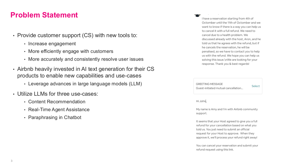
This slide lays out the problem statement for the Airbnb case study. The core goal is to provide customer support with new tools that increase engagement, handle customers more efficiently, and resolve issues more accurately and consistently. Airbnb invested heavily in AI text generation for their CS products to enable new capabilities, leveraging advances in large language models. They identified three specific use cases: content recommendation — matching users to the right help article, real-time agent assistance — suggesting appropriate responses to support agents in real time, and paraphrasing in chatbot — summarizing the user's problem back to them. The right side shows a real example: a customer writing about a reservation cancellation with a refund request, and the agent receiving a greeting message template to select and personalize. This gives you a concrete picture of what the system looks like in practice. These three use cases cover the main ways text generation can augment customer support at scale.

Before diving into Airbnb's solutions, here are some discussion questions to consider. First, why does it make sense for Airbnb to invest in these new AI text tools? Think about the scale of their customer support operations and the cost savings from even partial automation. Second, given what we've learned in class, what are some of the first baseline models you would try for each use case — content recommendation, selecting appropriate customer support response templates, and summarizing user problems? For content recommendation, you might start with a simple similarity model. For template selection, a basic classifier could work. For summarization, an extractive approach might be a reasonable baseline. Third, should Airbnb build or buy this technology, and which parts? This build-vs-buy decision is critical — back then, there weren't great off-the-shelf options, but today the landscape is very different with ChatGPT and other LLM APIs available.

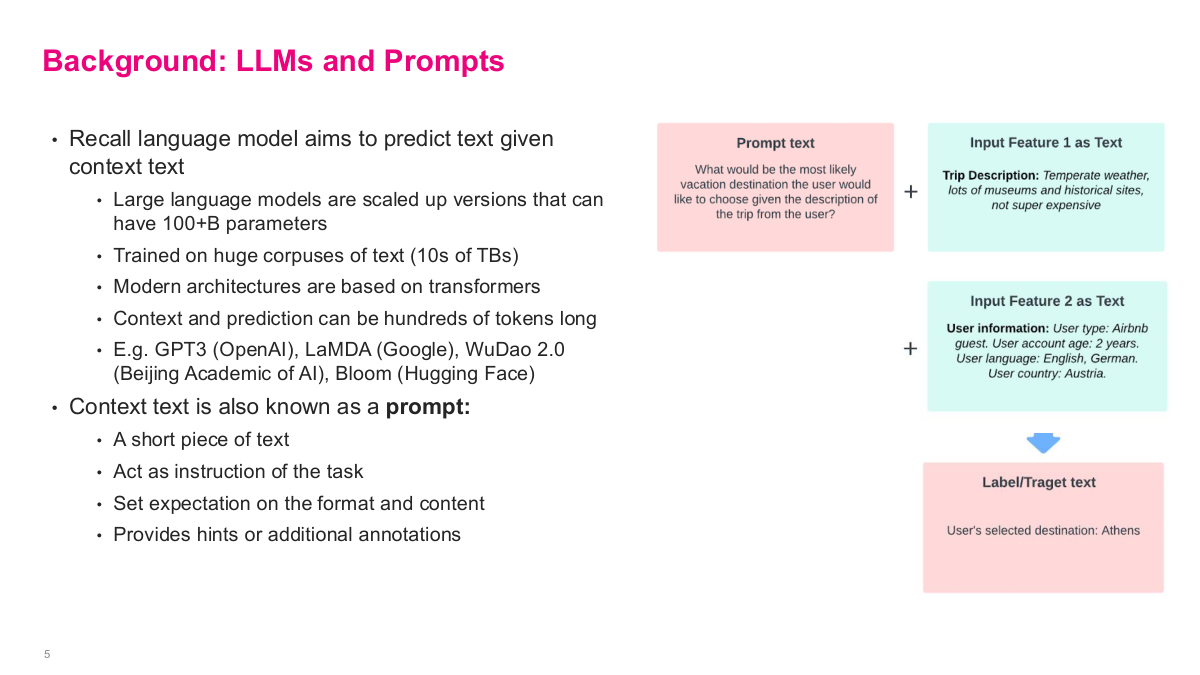
This slide provides background on LLMs and prompts that's essential for understanding Airbnb's approach. Recall that a language model aims to predict text given context text. Large language models are scaled up versions that can have 100+ billion parameters, trained on huge corpuses of text — tens of terabytes. Modern architectures are based on transformers, and context and prediction can be hundreds of tokens long. Examples include GPT-3 from OpenAI, LaMDA from Google, WuDao 2.0, and Bloom from Hugging Face. The context text is also known as a prompt — a short piece of text that acts as an instruction for the task, sets expectations on the format and content, and provides hints or additional annotations. The diagram on the right shows how Airbnb formulated this: they combine a prompt text with input features as text — like trip description and user information — and the model produces a label or target text. This is the fundamental pattern they used across their three use cases, treating everything as text-in, text-out.

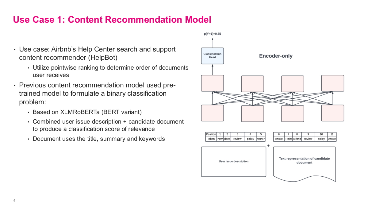
The first use case is content recommendation for Airbnb's Help Center search and support content recommender, called HelpBot. The approach uses pointwise ranking to determine the order of documents users receive. Their previous content recommendation model used a pre-trained model based on XLMRoBERTa, a BERT variant, to formulate a binary classification problem. They combined the user issue description with a candidate document — using the document's title, summary, and keywords — and fed both into an encoder-only architecture to produce a classification score of relevance. The key idea is that this is pointwise: for each candidate document, you run a separate forward pass through the model and get a probability score, like p(Y=1) = 0.85. Then you rank all candidates by their scores. It's a straightforward but effective approach — you're essentially asking "is this document relevant to this user's issue?" for each candidate independently, rather than trying to rank them all at once.

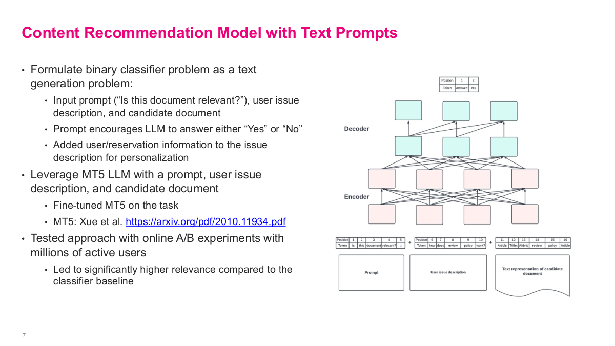
This slide shows the improved approach: formulating the binary classifier problem as a text generation problem instead. They use an input prompt like "Is this document relevant?", along with the user issue description and candidate document, and the prompt encourages the LLM to answer either "Yes" or "No." They also added user and reservation information to the issue description for personalization. They leveraged the MT5 LLM — a massively multilingual pre-trained text-to-text transformer — with the prompt, user issue, and candidate document fed into an encoder-decoder architecture. They fine-tuned MT5 on this task. The results were impressive: they tested this approach with online A/B experiments with millions of active users, and it led to significantly higher relevance compared to the classifier baseline. Using the LLM essentially as a classifier yielded much better results than having it directly generate answers — an interesting pattern worth trying even with modern LLMs when accuracy matters.

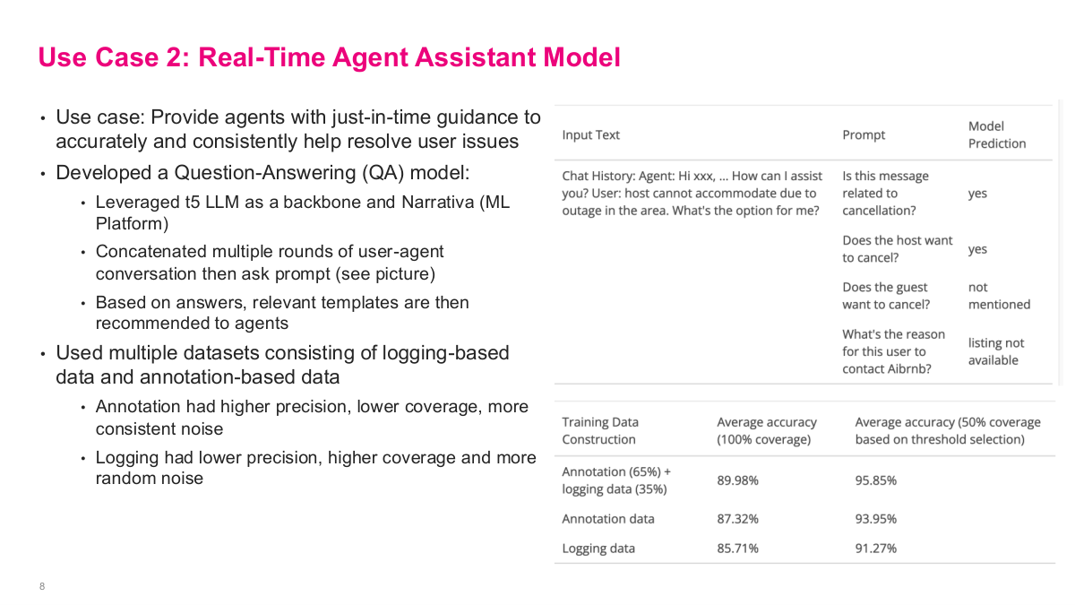
The second use case is a real-time agent assistant model. The goal is to provide agents with just-in-time guidance to accurately and consistently help resolve user issues. They developed a question-answering model, leveraging T5 LLM as a backbone along with Narrativa, their ML platform. The approach concatenates multiple rounds of user-agent conversation, then asks a prompt — you can see the example on the right showing questions like "Is this message related to cancellation?" or "Does the host want to cancel?" Based on the model's answers, relevant templates are recommended to agents. For training data, they used multiple datasets consisting of logging-based data and annotation-based data. The annotation data had higher precision but lower coverage with more consistent noise, while logging data had lower precision but higher coverage with more random noise. Combining both — 65% annotation plus 35% logging — gave the best results at about 90% average accuracy, outperforming either source alone.

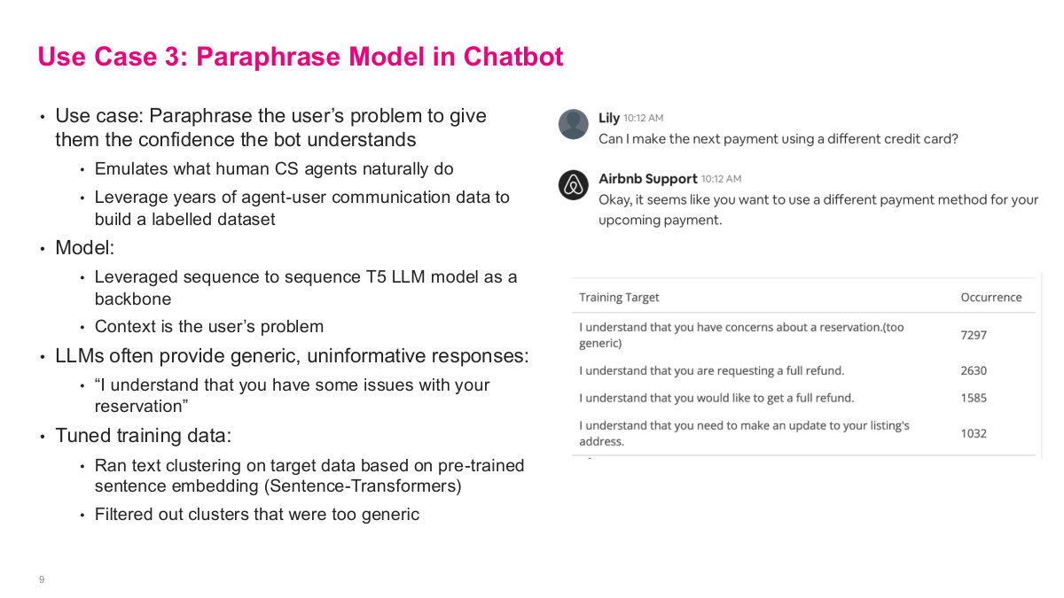
The third use case is the paraphrase model in chatbot. The goal is to paraphrase the user's problem to give them confidence the bot understands — emulating what human CS agents naturally do. They leveraged years of agent-user communication data to build a labelled dataset. The model used a sequence-to-sequence T5 LLM as a backbone, with the user's problem as context. But LLMs often provide generic, uninformative responses like "I understand that you have some issues with your reservation" — you can see in the training target table that this generic response occurred 7,297 times, dominating the dataset. To fix this, they tuned the training data by running text clustering on the target data based on pre-trained sentence embeddings from Sentence-Transformers, then filtered out clusters that were too generic. This is a really important pattern — rather than trying to fix the model directly, they fixed the dataset. By cleaning the fine-tuning data this way, the T5 model stopped producing those boilerplate answers and generated more specific, useful paraphrases.

This references slide closes the Airbnb customer-support case study and points back to the original engineering write-up. It is worth reading directly because the details on prompt design, data preparation, and online evaluation are more specific than what we can cover in class.

Our next use case shifts from NLP to a more direct prediction problem — how Uber predicts arrival times using deep learning. This is DeepETA, and it's a fascinating problem because estimated arrival times power so many Uber experiences: rides, freight, Eats — dispatch, navigation, fares, and many more. When you request a ride, Uber needs to tell you when the driver will arrive, and getting that estimate right is critical for customer satisfaction and for accurately calculating fares. The problem is deceptively hard because it depends on traffic patterns, road conditions, driver behavior, time of day, and countless other factors that interact in non-linear ways — making it a natural fit for deep learning approaches.

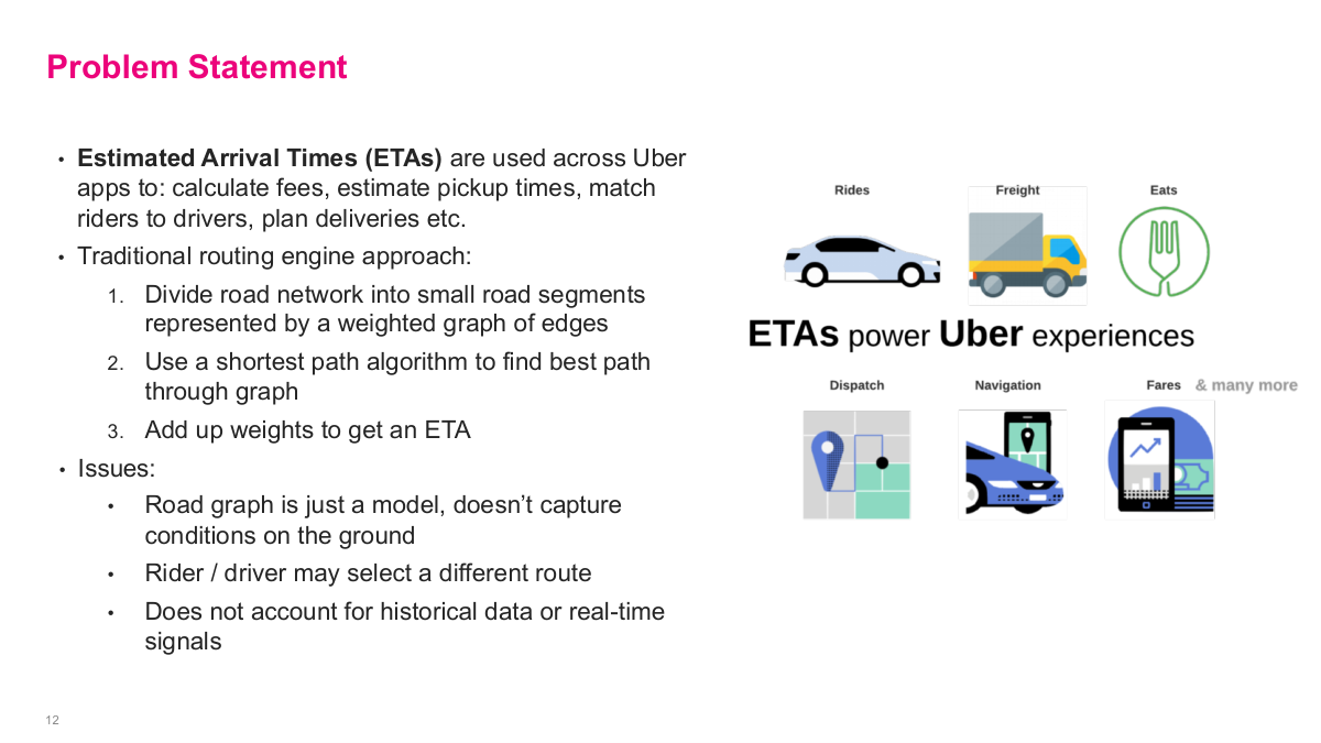
This slide lays out the problem statement for the Uber ETA case. Estimated arrival times are used across all Uber apps to calculate fees, estimate pickup times, match riders to drivers, plan deliveries, and more. The traditional routing engine approach divides the road network into small road segments represented by a weighted graph of edges, uses a shortest path algorithm to find the best path through the graph, then adds up the weights to get an ETA. But there are fundamental issues with this approach. The road graph is just a model — it doesn't capture real conditions on the ground. The rider or driver may select a different route than what was predicted. And it doesn't account for historical data or real-time signals like traffic, weather, or events. So what data could improve on a basic routing engine? Traffic data, weather conditions, historical trip times, driver behavior — the richness of available data far exceeds what a traditional segment-based routing engine can leverage.

Here are some discussion questions for the Uber case. What data could they use that the traditional routing engine approach doesn't take advantage of? Think about traffic data, weather, historical patterns, driver behavior, and real-time signals. What are some of the main metrics to optimize for ETAs? Accuracy is obvious, but latency matters enormously — the estimate needs to be computed fast enough to be useful. Generality is important too since Uber operates across many different markets worldwide. And cost is a real constraint — you don't want to invest a billion dollars building this system if the improvement doesn't justify it. How would you formulate the ML problem? Given that you already have an existing routing system, how do you frame where ML fits in? And what are some production considerations when serving tens or hundreds of millions of customers worldwide? These questions frame the engineering challenge that drives the entire DeepETA project.

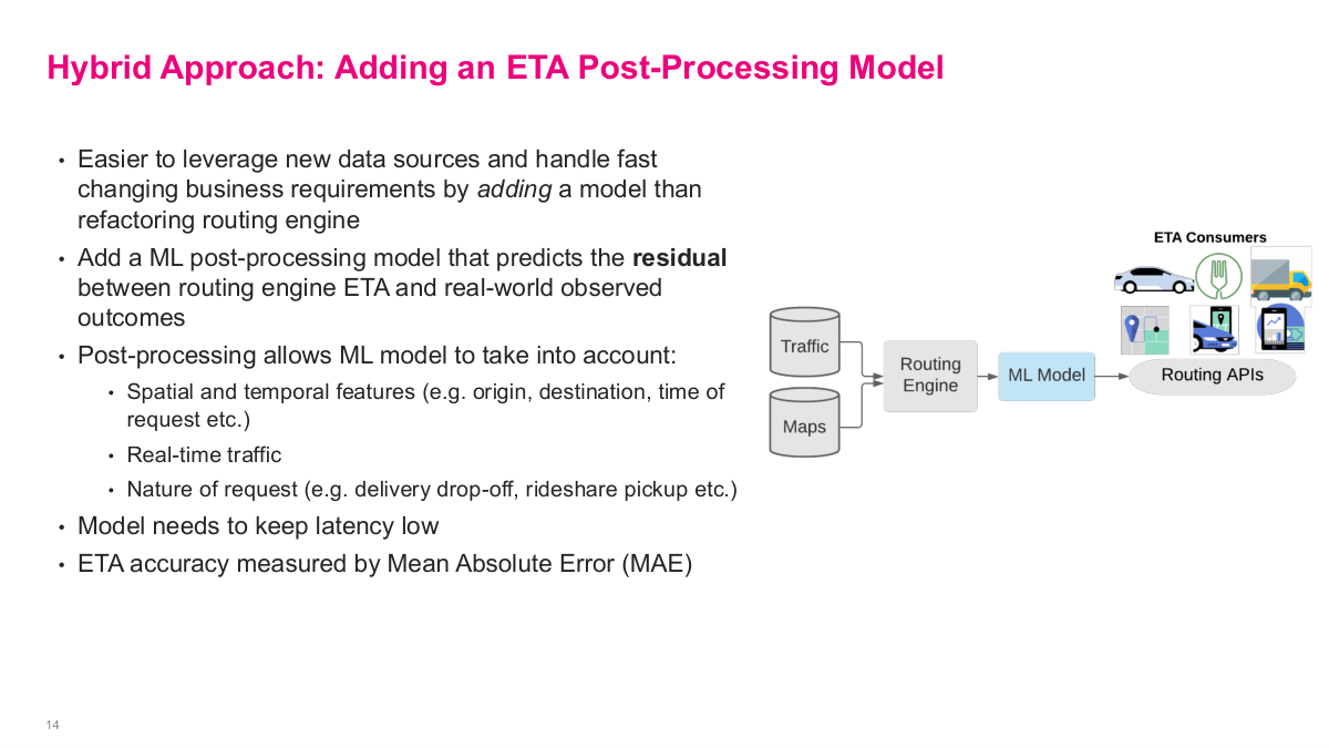
Uber's solution is elegant — a hybrid approach. Rather than replacing the traditional routing engine, they add an ML post-processing model on top. It's easier to leverage new data sources and handle fast-changing business requirements by adding a model than refactoring the routing engine itself. The ML model predicts the residual — the difference between the routing engine's ETA and real-world observed outcomes. This post-processing allows the ML model to take into account spatial and temporal features like origin, destination, and time of request, real-time traffic conditions, and the nature of the request such as delivery drop-off versus rideshare pickup. The model needs to keep latency low since users are waiting for the estimate. ETA accuracy is measured by mean absolute error. The diagram shows the architecture: traffic and maps data feed into the routing engine, then the ML model corrects its output before the result goes to routing APIs and ultimately to ETA consumers.

The first version of the ML post-processing model used gradient boosted decision tree ensembles — specifically XGBoost, a sensible choice for tabular data. But as the model and training dataset grew steadily larger with each release, they needed to leverage Apache Spark to process massive amounts of data and train distributed XGBoost models. At some point, training XGBoost with large dataset sizes became untenable even with distributed infrastructure across hundreds of servers. So they considered switching to a deep learning model because of the ease of scaling distributed training to large datasets. But they needed to overcome three main challenges: latency — they need to return a result in a few milliseconds as most, accuracy — it needs to significantly improve the metric (MAE) to justify the cost, and generality — it needs to be able to predict across all of Uber's businesses. This motivated the development of DeepETA.

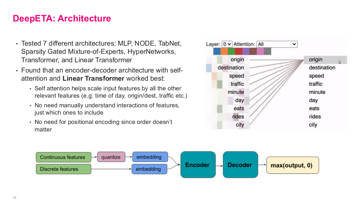
This slide shows the DeepETA architecture. They tested 7 different architectures — MLP, NODE, TabNet, Sparsity Gated Mixture-of-Experts, HyperNetworks, Transformer, and Linear Transformer. They found that an encoder-decoder architecture with self-attention and a Linear Transformer worked best. Self-attention helps scale input features by all the other relevant features — time of day, origin/destination, traffic — without needing to manually understand interactions of features, just which ones to include. There's no need for positional encoding since feature order doesn't matter. The attention visualization on the right shows how features like origin, destination, speed, and traffic interact with each other. For feature encoding, continuous features are quantized into buckets then embedded, while discrete features go directly to embeddings. Everything feeds into the encoder, then the decoder produces a prediction with max(output, 0) to ensure non-negative values. This is the recommended first step in any deep learning effort — define your benchmark set, selection criteria, test metrics, and evaluate multiple architectures before committing to one.

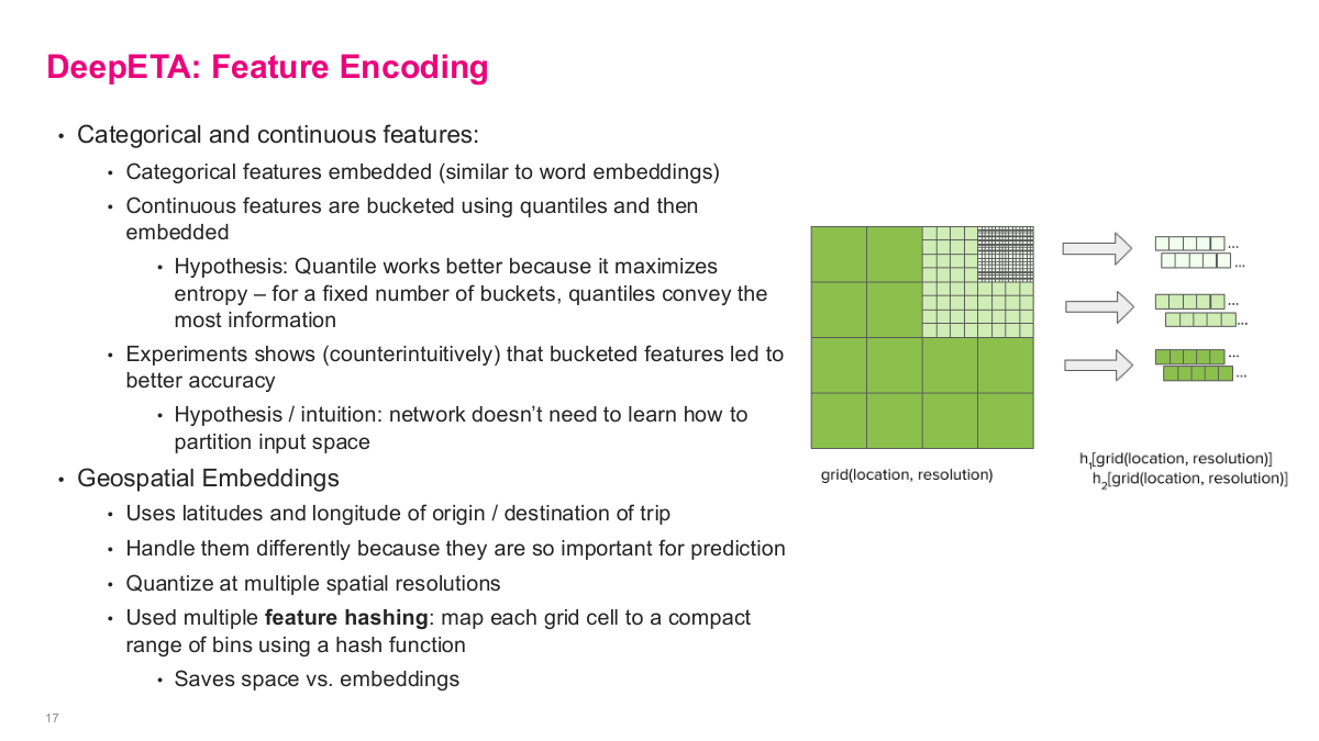
This slide dives into DeepETA's feature encoding, which is crucial for performance. For categorical and continuous features: categorical features are embedded similar to word embeddings — standard practice. But for continuous features, they're bucketed using quantiles and then embedded. The hypothesis is that quantile bucketing works better because it maximizes entropy — for a fixed number of buckets, quantiles convey the most information. Experiments showed counterintuitively that bucketed features led to better accuracy, because the network doesn't need to learn how to partition the input space on its own. For geospatial embeddings, they handle latitudes and longitudes of origin and destination differently because they're so important for prediction. They quantize at multiple spatial resolutions and use feature hashing — mapping each grid cell to a compact range of bins using a hash function, which saves space versus full embeddings. The visualization shows how the same location gets encoded at coarse, medium, and fine resolution levels. This multi-resolution approach lets the model capture geographic patterns at different scales.

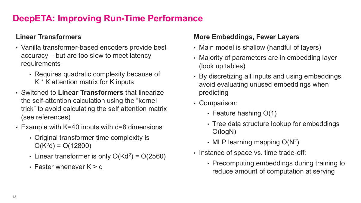
Several clever techniques improved DeepETA's runtime performance. First, linear transformers. Full transformers predicted slightly better but were too slow. Standard transformer computation scales quadratically with sequence length — k-squared times d. Linear transformers use an approximation that scales as k times d-squared instead. When k is large and d is small (like 8), linear transformers are much faster. Accuracy isn't everything; latency constraints may dictate architecture choices.

Second, they pre-computed embeddings for discrete variables during training, then cached them in lookup tables. Instead of computing embeddings on the fly with O(n²) cost, they achieved O(1) lookup via hash tables — a smart space-versus-time tradeoff.

Third, a segment bias layer in the decoder adapted the base model to different regions, similar to transfer learning with adapters.

Fourth, they used asymmetric Huber loss because arriving late is worse than arriving early. The piecewise loss function penalizes late predictions more heavily, biasing estimates to be slightly early. Custom loss functions tailored to business objectives are a powerful technique.

Finally, Uber's internal Michelangelo platform handles auto-retraining, validation, and serving the model via API at scale.

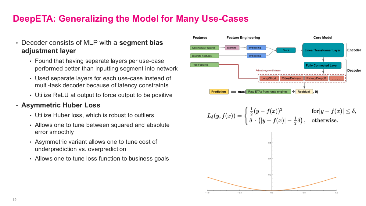
This slide covers how DeepETA generalizes across Uber's many use cases. The decoder consists of an MLP with a segment bias adjustment layer. They found that having separate layers per use case performed better than inputting segment type into the network. They used separate layers for each use case instead of a multi-task decoder because of latency constraints, and utilized ReLU at the output to force predictions to be positive. A key innovation is asymmetric Huber loss. They use Huber loss because it's robust to outliers — it allows you to tune between squared and absolute error smoothly. The asymmetric variant lets you tune the cost of underprediction versus overprediction, which makes sense because arriving late is worse than arriving early from a user experience perspective. This allows you to tune the loss function to business goals. The diagram shows the full architecture: continuous features get quantized then embedded, discrete features get embedded directly, type features go through separate segment bias layers in the decoder for Long/Short, Rides/Delivery, Pickup/Dropoff, and the final prediction combines the raw ETA from route engines with the learned residual.

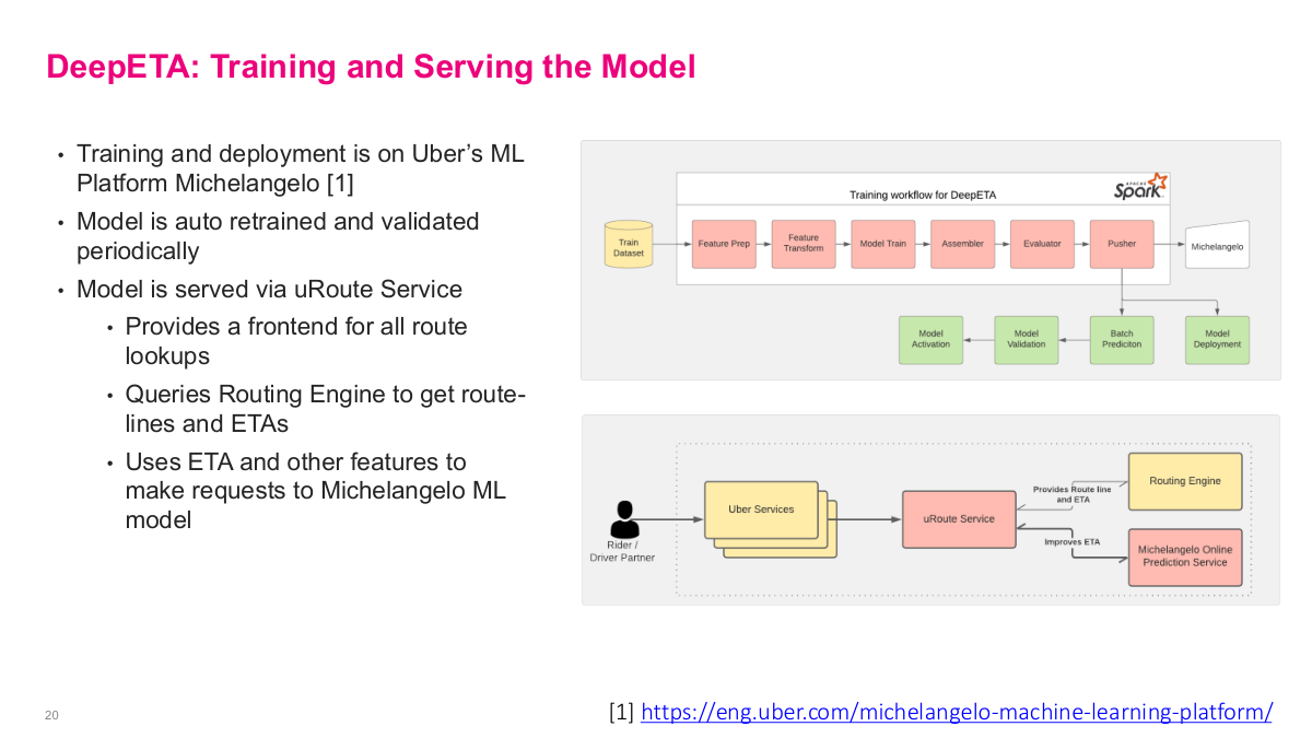
This slide covers training and serving for the DeepETA model. Training and deployment runs on Uber's ML platform Michelangelo. The model is auto-retrained and validated periodically — critical for keeping predictions fresh as traffic patterns change. The training workflow goes through feature prep, feature transform, model train, assembler, evaluator, pusher, then into Michelangelo for model activation, validation, batch prediction, and model deployment. The model is served via the uRoute Service, which provides a frontend for all route lookups, queries the routing engine to get route-lines and ETAs, then uses the ETA and other features to make requests to the Michelangelo ML model to improve the ETA estimate. This architecture shows the full production pipeline — from a rider or driver partner making a request through Uber Services, to uRoute Service, which queries both the routing engine and the Michelangelo online prediction service to produce the final corrected ETA.

This references slide wraps up the Uber DeepETA case study. The main value of the original post is not just the final model, but the production details around feature design, latency constraints, architecture choices, and deployment on a real ML platform.

Now we shift to a computer vision use case: amenity detection at Airbnb. Airbnb cares deeply about listing photos because they significantly impact conversion rates and bookings. The specific problem is that hosts often don't list every amenity their property has. Amenity detection is a popular problem in computer vision called object detection. Their first instinct was correctly to look at third-party APIs or open-source implementations — why reinvent the wheel? But the challenge was that generic 3rd party vendors only offer generic object detection. Open source projects also had pre-trained object detection models, but their prediction was low and predicted labels were often incorrect for Airbnb's needs. Airbnb needed specific labels like "kitchen," "dining table," "refrigerator" — not just "table" and "kitchenware." So the requirements were clear: they needed a custom set of amenity labels, an image dataset with annotations, and reasonable accuracy before putting it in front of users.

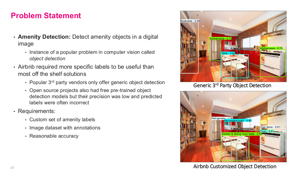
This slide frames the amenity detection problem statement. Amenity detection means detecting amenity objects in a digital image — it's a popular problem in computer vision called object detection. Airbnb required more specific labels to be useful than most off-the-shelf solutions provide. Popular 3rd party vendors only offer generic object detection, and open source projects also had pre-trained models but their precision was low and labels were often incorrect for Airbnb's specific needs. The requirements boil down to: a custom set of amenity labels, an image dataset with annotations for training, and reasonable accuracy. The images on the right show the difference — a generic 3rd party object detection model labels things broadly, while Airbnb's customized object detection identifies specific amenities like kitchen appliances and furniture that matter for listings.

Before diving into Airbnb's solution, here are some discussion questions for the amenity detection case. First, why was their first choice to look for a 3rd party API or open source implementations? This gets at the build-vs-buy decision — in a space with lots of existing work, you should always check what's available before building from scratch. Second, how would you go about building a label taxonomy? This is a non-trivial problem — you need to define the universe of amenity categories that are both useful to users and feasible to detect. Third, how would you go about collecting an annotated dataset? Getting labeled data is often the hardest and most time-consuming part of any supervised learning project. These questions frame the practical engineering challenges that Airbnb had to solve before they could even think about model architecture.

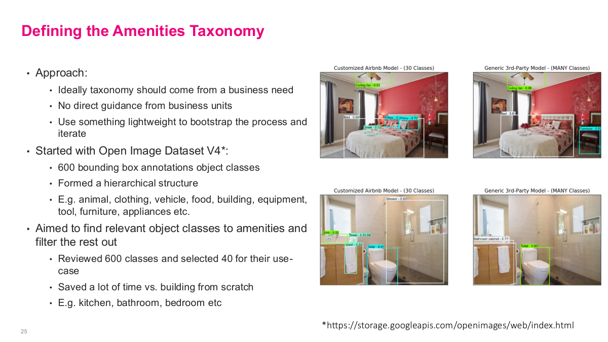
This slide covers how Airbnb defined their amenities taxonomy. Their approach started with the idea that the taxonomy should come from a business need — ideally direct guidance from business units. They used something lightweight to bootstrap the process and iterate. They started with Open Image Dataset V4, which has about 600 bounding box annotation object classes. They formed a hierarchical structure with categories like animal, clothing, vehicle, food, furniture, appliance, etc. Then they aimed to find relevant object classes for amenities and filter the rest out — they reviewed 600 classes and selected 40 for their use case. This saved a lot of time versus building a taxonomy from scratch. For example, they'd keep labels like kitchen, bathroom, swimming pool, dining table, refrigerator, and microwave, while filtering out irrelevant ones like animal or vehicle. Getting the taxonomy right is the essential first step before you can build a training dataset.

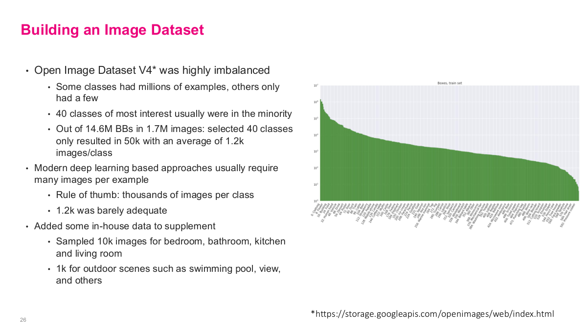
This slide covers building the image dataset. The Open Image Dataset V4 was highly imbalanced — some classes had millions of examples, others only had a few. The 40 classes of most interest were usually in the minority. Out of 14.6 million bounding boxes in 1.7 million images, their selected 40 classes only resulted in 50,000 images with an average of about 1,200 images per class. Modern deep learning approaches usually require many images per example — the rule of thumb is thousands of images per class, and 1,200 was barely adequate. To supplement, they added in-house data from Airbnb's own image repository — they sampled 10,000 images for bedrooms, bathrooms, kitchens, and living rooms, plus 1,000 for outdoor scenes like swimming pools and views. This combination of open-source data with proprietary listing images gave them enough to actually train a model.

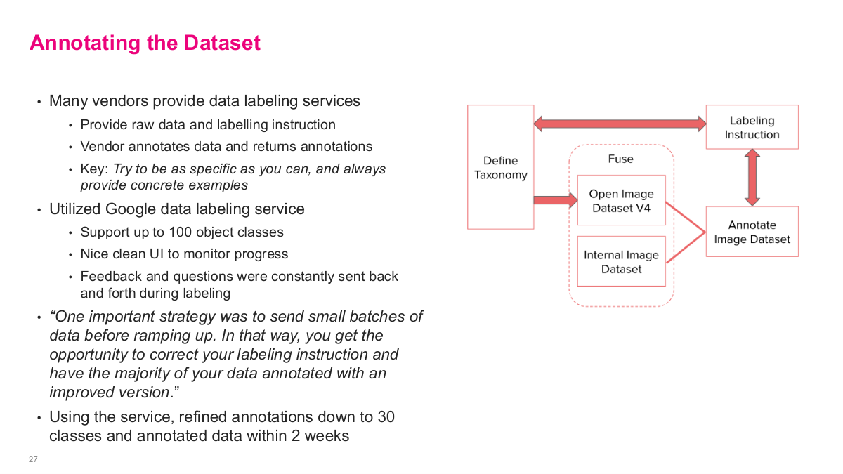
This slide covers annotating the dataset. Many vendors provide data labeling services — you provide raw data and labeling instructions, and the vendor annotates data and returns annotations. The key is to try to be as specific as you can and always provide concrete examples. They utilized Google's data labeling service, which supports up to 100 object classes, has a nice clean UI to monitor progress, and allows feedback and questions to be constantly sent back and forth during labeling. One important strategy was to send small batches of data before ramping up — that way you get the opportunity to correct your labeling instructions and have the majority of your data annotated with an improved version. Using this service, they refined annotations down to 30 classes and annotated data within 2 weeks. The diagram shows the pipeline: define taxonomy, fuse with Open Image Dataset V4 and internal image dataset, create labeling instructions, and iterate on the annotated image dataset.

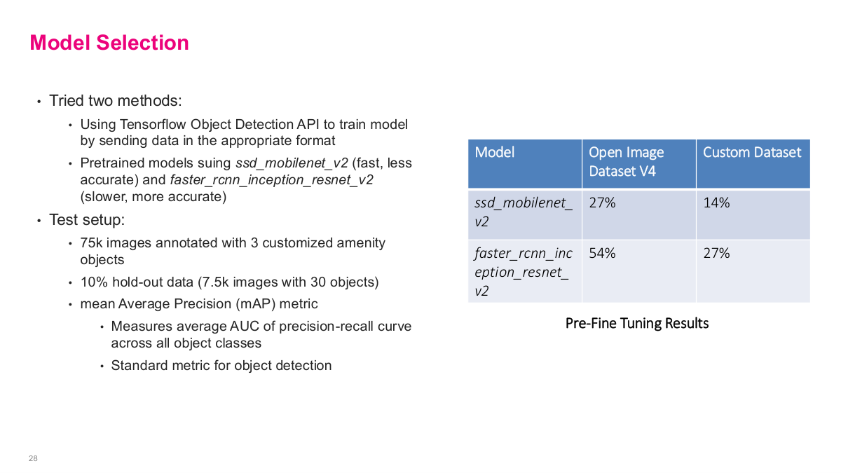
This slide covers model selection. They tried two methods using the TensorFlow Object Detection API. They used pretrained models: ssd_mobilenet_v2, which is fast but less accurate, and faster_rcnn_inception_resnet_v2, which is slower but more accurate. The test setup used 75,000 images annotated with 3 customized amenity objects, with a 10% hold-out data set of 7,500 images with 30 objects. They used mean average precision (mAP) as their primary metric — it measures the average AUC of the precision-recall curve across all object classes, and it's the standard metric for object detection. The pre-fine-tuning results showed that on the Open Image Dataset, ssd_mobilenet_v2 got 27% mAP and faster_rcnn_inception_resnet_v2 got 54%, while on their custom dataset the scores were 14% and 27% respectively. These baseline numbers set the stage for fine-tuning.

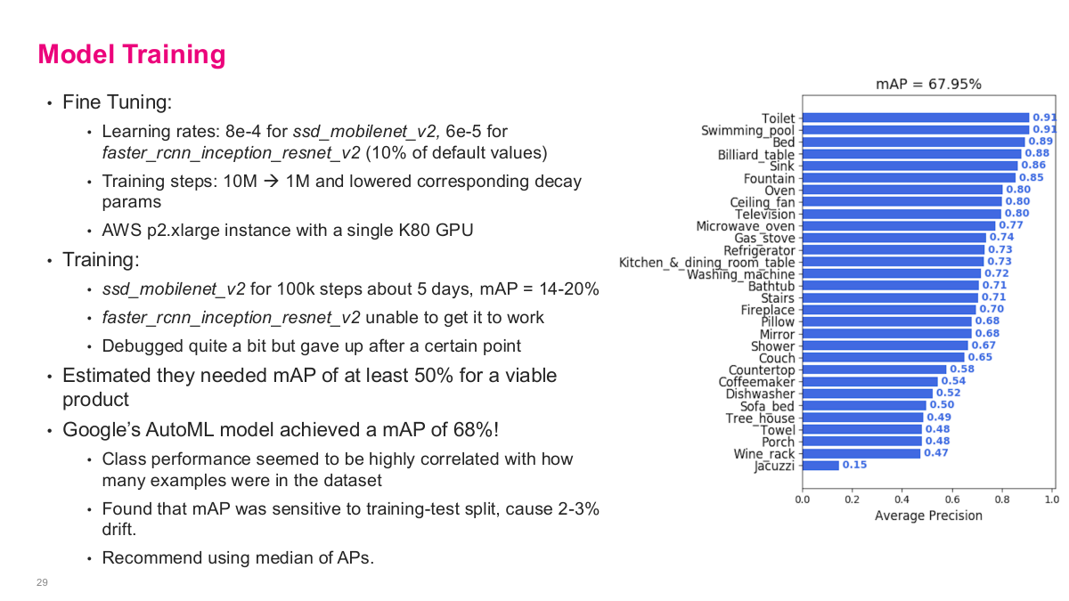
This slide shows the model training results. For fine-tuning, they used learning rates of 8e-4 for ssd_mobilenet_v2 and 6e-5 for faster_rcnn_inception_resnet_v2, with training steps reduced from 10M to 1M with lowered decay params on an AWS p2.xlarge instance with a single K80 GPU. The ssd_mobilenet_v2 ran for 100k steps over about 5 days and achieved a mAP of 14-20%. The faster_rcnn_inception_resnet_v2 was unable to get working — they debugged quite a bit but gave up after a certain point. They estimated they needed at least 50% mAP for a viable product. The big surprise: Google's AutoML model achieved a mAP of 68%! Class performance was highly correlated with how many examples were in the dataset. They found mAP was sensitive to the training-test split, causing 2-3% drift, and recommend using median of average precisions. The bar chart shows per-class performance ranging from toilets at 0.93 down to jacuzzi at 0.15.

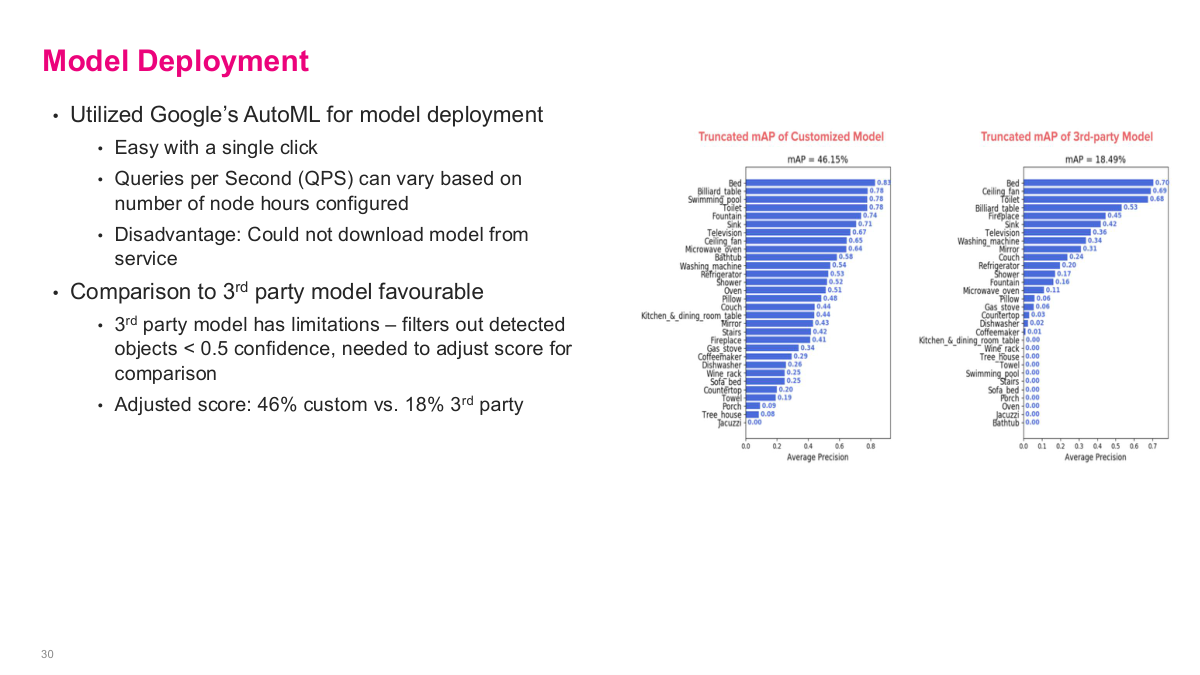
For model deployment, they utilized Google's AutoML, which made it easy with a single click. Queries per second can vary based on the number of node hours configured, giving them scalable serving. The disadvantage is that you cannot download the model from the service — you're locked into Google's infrastructure. The comparison to 3rd party models was favourable. The 3rd party model has limitations — it filters out detected objects below 0.5 confidence, so they needed to adjust scores for comparison. The adjusted scores showed their custom model at 46% truncated mAP versus 18% for the 3rd party model — a substantial improvement. Google's AutoML actually outperformed anything the team could build in-house, and the off-the-shelf solution was simply better. The key takeaway is that most of the real work wasn't on the ML model itself — it was on formulating the problem in terms of taxonomy, assembling and cleaning the data, then leveraging off-the-shelf tools for what was probably industry-leading accuracy.

This slide summarizes the lessons learned from the amenity detection case study. First, data is more important than the model — you'll probably spend 90% of your time collecting and parsing big chunks of data. Second, be creative when gathering data and don't reinvent the wheel — leverage public data from the open source community when possible and integrate it with your private data if necessary. Third, getting high-quality labels for your data is almost always the most critical step for a supervised model — labeling is often the most time-consuming process with lots of coordination between organizations. Plan early and choose a vendor for annotations wisely. Fourth, using a good machine learning tool can significantly speed up your model training and deployment — as demonstrated by AutoML outperforming their manual efforts. Fifth, be open-minded — don't be afraid to start with a simple solution, even if it's just a generic third-party API. It may not solve your business problem immediately, but will likely lead to a successful solution sometime later.

Now we shift to a Slack case study on personalized channel recommendations. When you join Slack or at various points during usage, they want to recommend channels that are most relevant to you via Slackbot. The fundamental challenge is there's no direct way to measure if a channel is relevant — there's no "I like this channel" button. They settled on time spent in the channel based on read/write activity as their proxy metric. The user-channel matrix can have millions of entries — potentially 100,000 users times 10,000 channels. They formulated it as a classic matrix completion recommendation problem: build this user-channel matrix, estimate relevancy scores, use a test set consisting of a random subset of filled entries plus a random sample of empty cells with activity = 0. The matrix diagram shows channels C1-C3 and users U1-U3, with some cells filled with activity scores and others empty — the goal is to predict the empty cells.

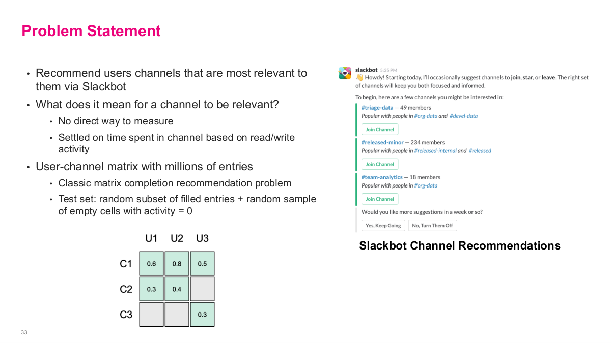
This is the problem statement for the Slack channel recommendations case. The goal is to recommend users channels that are most relevant to them via Slackbot. What does it mean for a channel to be relevant? There's no direct way to measure it, so they settled on time spent in the channel based on read/write activity as a proxy metric. The user-channel matrix has millions of entries, making it a classic matrix completion recommendation problem. The test set consists of a random subset of filled entries plus a random sample of empty cells with activity equal to zero. The slide shows the matrix structure: channels as rows, users as columns, with some cells filled with activity scores like 0.6, 0.8, 0.5 and others empty. The right side shows the actual Slackbot experience — it suggests channels like #triage-data and #released-minor with a "Join Channel" button, along with which channels' members overlap with yours. Users can opt to keep getting suggestions or turn them off.

Here are the discussion questions for the Slack case. What other metrics might you measure relevancy besides activity time? Think about reactions, message frequency, return visits, or admin roles. What recommendation system approaches would you try? We learned several — latent factor models, collaborative filtering, item-based similarity. Does the data size limit the techniques we can use? With maybe 10,000 channels, the similarity matrix is 10,000 squared — about 100 million entries, which is actually manageable on a modern laptop. How would your approach change if you only have 3 months to build a prototype? Sometimes quick and dirty is the right strategy to prove value. What other tasks do you need to do to build out this feature? Think about UI design, serving infrastructure, A/B testing. And how would you measure the efficacy of the final released feature? These questions frame the practical engineering and product decisions that go beyond just the ML model.

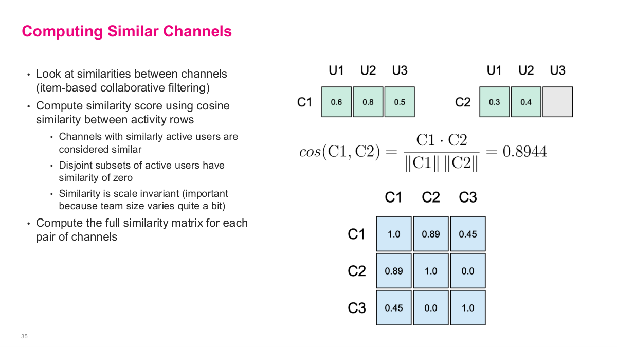
Slack's approach was to look at similarities between channels — item-based collaborative filtering. They compute a similarity score using cosine similarity between activity rows. Channels with similarly active users are considered similar, disjoint subsets of active users have similarity of zero, and the similarity is scale invariant — important because team size varies quite a bit across channels. They compute the full similarity matrix for each pair of channels. The slide shows the math: take channels C1 and C2 with their user activity vectors, compute cosine similarity as the dot product divided by the product of norms, yielding 0.8944 in the example. The resulting channel-channel similarity matrix has values like C1-C2 = 0.89, C1-C3 = 0.45, and C2-C3 = 0.0 — which makes sense because C2 and C3 share no active users. This is entirely an offline computation that you build once and reference when generating recommendations.

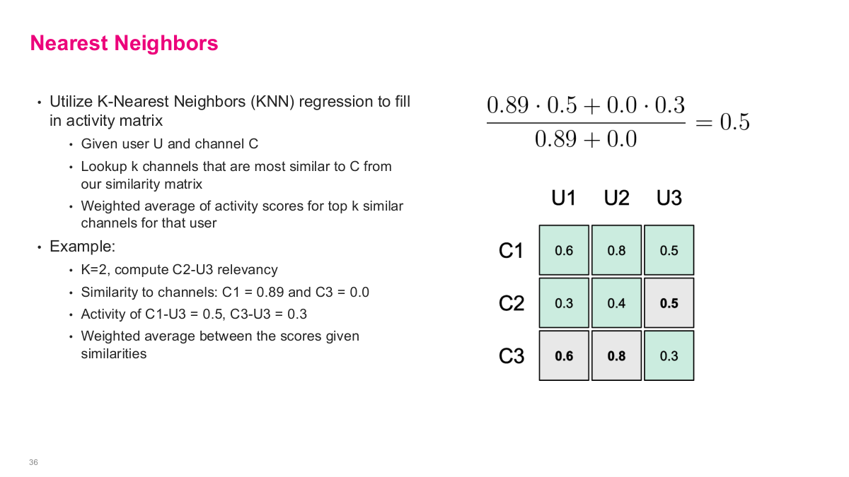
With the similarity matrix built, they use K-Nearest Neighbors regression to fill in the missing user-channel relevancy scores. Given a user U and channel C, you look up the k channels that are most similar to C from the similarity matrix, then compute a weighted average of activity scores for the top k similar channels for that user. The example on the slide shows this clearly: with K=2, to compute the relevancy of C2 for U3, they find the similarity of C2 to other channels — C1 similarity is 0.89 and C3 is 0.0. Then they take the activity scores: C1-U3 = 0.5 and C3-U3 = 0.3. The weighted average is (0.89 0.5 + 0.0 0.3) / (0.89 + 0.0) = 0.5. This fills in the previously empty cell. This is exactly the collaborative filtering heuristic we discussed in an earlier lecture — using weighted averages of similar items to estimate missing values.

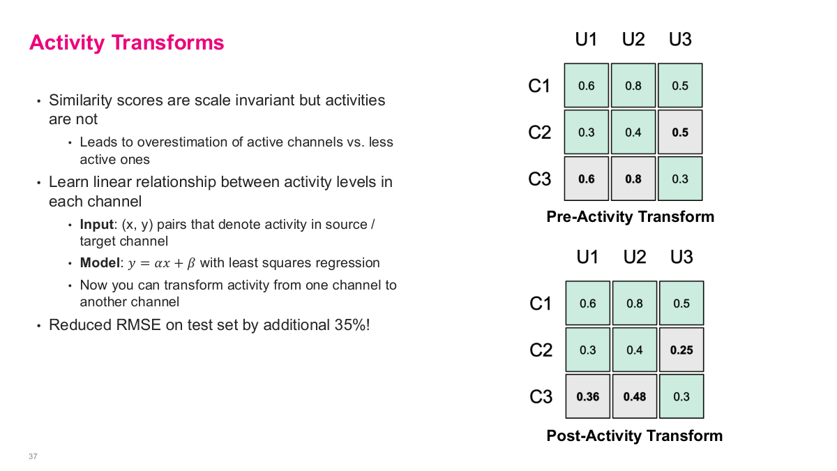
This slide introduces activity transforms, which address a key problem: while similarity scores are scale invariant, the activity values themselves are not. This leads to overestimation of active channels versus less active ones. The solution is to learn a linear relationship between activity levels in each channel. The input is (x, y) pairs that denote activity in the source versus target channel, and the model is y = αx + β fitted with least squares regression. Now you can transform activity from one channel to another, normalizing for the fact that some channels are inherently more active than others. The slide shows the before and after: in the pre-activity transform matrix, the raw KNN prediction for C2-U3 is 0.5, but after applying the activity transform, it's adjusted down to 0.25. Similarly, the empty cells for C3 get filled with transformed values of 0.36 and 0.48. This single adjustment reduced RMSE on their test set by an additional 35% — a significant improvement from a simple normalization step.

Beyond the model, many additional tasks were needed before the feature could be rolled out. They had to design how recommendations were displayed, build infrastructure to index and serve recommendations, choose the wording and interaction model used by Slackbot, implement triggering logic so it wouldn't be distruptive, and quantify success using Slack's internal experiment and logging system. The results: a 22% click-through rate for recommendations — meaningful impact from a simple approach. Future work involves a larger regression model that leverages more features. The key takeaway from this case study is that a simple, well-reasoned approach delivered real business value. Unless you're operating at massive scale, chasing the last 20% improvement with complex models often isn't worth the engineering investment. The 80/20 rule applies strongly here — start simple, prove value, then iterate.

Now we shift to our final case study: DoorDash optimizing marketing spend with machine learning. This is a critical problem for companies that invest heavily in user acquisition across platforms like Facebook and Google. Marketing campaigns are managed by an internal team per channel, with well-performing campaigns being boosted and underperforming ones turned off. There can be over 10,000 campaigns active at any given time. They programmatically built a marketing automation platform to operate at this scale — the ML system optimally allocates budget to each campaign and bids to channel partners.

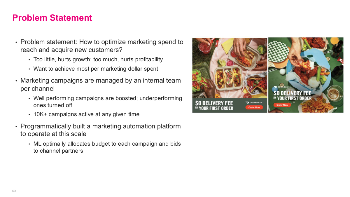
This slide frames the DoorDash problem statement. How do you optimize marketing spend to reach and acquire new customers? The top-line goals are to grow, get more users, increase profitability — essentially maximize the return on every marketing dollar spent. Marketing campaigns are managed by an internal team per channel, and there can be over 10,000 campaigns active at any given time. The images on the right show typical DoorDash promotional offers — delivery fee discounts and new customer signup incentives. The core optimization question is: given a fixed total marketing budget, how do you allocate spend across thousands of campaigns and channels to maximize conversions? This requires understanding the cost curve for each campaign — how conversions scale with spending — which is where ML comes in.

Here are the discussion questions for the DoorDash case. What types of data would you need to analyze marketing budgets? Think about spend per campaign, conversion rates, impression counts, click-through rates, and campaign metadata like targeting, format, and region. How do you deal with sparse data? This is a real challenge because some campaigns are very small with few data points, while others have concentrated data in narrow spend ranges. What types of models deal well with sparse data? These questions frame the core technical challenges — estimating cost curves from limited, unevenly distributed data across thousands of campaigns is fundamentally harder than having a nice clean dataset to work with.

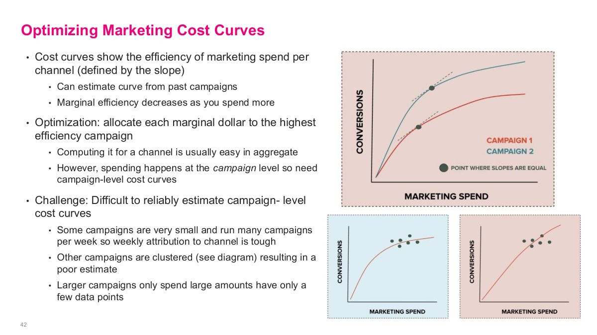
Cost curves show the efficiency of marketing spend per channel, defined by the slope — as you spend more, marginal efficiency decreases because you saturate the engaged audience. You can estimate the curve from past campaigns. The optimization goal is to allocate each marginal dollar to the highest efficiency campaign. However, spending happens at the campaign level, so you need campaign-level cost curves, not just channel-level aggregates. The challenge is that it's difficult to reliably estimate campaign-level cost curves from sparse data. Some campaigns are very small and run for a short time with few data points. Other campaigns are clustered — similar targeting, format, and bidding strategy — resulting in data concentrated in narrow spend ranges. Larger campaigns only spend large amounts, so you rarely have data for what would happen at low spend levels. Estimating these curves accurately from sparse, unevenly distributed data is the core technical challenge that drives the entire ML approach.

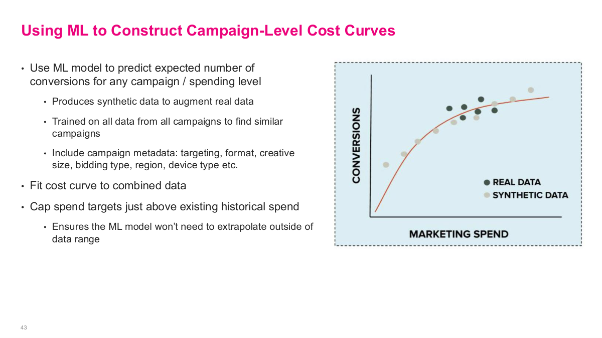
The key idea here is to use machine learning to estimate a campaign-level cost curve even when the real campaign data is sparse or clustered in only part of the spend range. DoorDash trains a model on data from many campaigns, uses campaign metadata to identify similar campaigns, generates synthetic points around the historical operating region, and then fits a smooth response curve to the combined real and synthetic data. The important guardrail is that they do not extrapolate too far beyond the historical spend range. This turns a messy sparse-data problem into a tractable optimization problem.

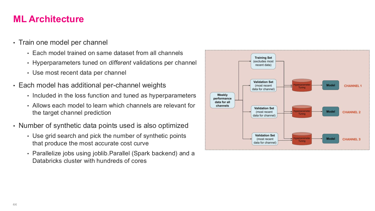
The architecture is interesting because it is neither a single global model nor a completely separate model per campaign. They train one model per channel, but each model still learns from the full training data across channels. What changes per channel is the validation set, the hyperparameter tuning, the per-channel weighting in the loss, and even the number of synthetic points used to construct the cost curve. It is a pragmatic setup: share as much data as possible, then specialize the model where it matters for the target channel. That kind of hybrid design shows up often in production ML systems.

This references slide closes the DoorDash marketing-spend case study and points to the original article. The write-up is useful because it shows how much of the work was in problem formulation, sparse-data handling, and production optimization rather than in choosing a flashy model.